Sequence Model (many-to-one) with Attention#
This is many-to-one sequence model
Matthew McAteer’s Getting started with Attention for Classification: A quick guide on how to start using Attention in your NLP models
This tutorial demonstrates a bi-directional LSTM sequence on sentiment analysis (binary classification). The key is to add Attention layer to make use of all output states from the bi-directional LSTMs. (Traditional LSTMs use only the final encoded state of the RNN for a prediction task.
The conundrum with RNNs/LSTMs is that they are not good at dealing with dependencies and relevant relationships in the previous steps of the sequences.
from importlib import  reload
import sys
from imp import  reload
import warnings
warnings.filterwarnings('ignore')
# if sys.version[0] == '2':
#     reload(sys)
# sys.setdefaultencoding("utf-8")

import nltk
# nltk.download('stopwords')
# nltk.download('wordnet')

import re
from nltk.stem import WordNetLemmatizer
from nltk.corpus import stopwords

import tensorflow as tf
import tensorflow.keras as keras
from tensorflow.keras.preprocessing.text import Tokenizer
from tensorflow.keras.preprocessing.sequence import pad_sequences
from tensorflow.keras.layers import Concatenate, Dense, Input, LSTM, Embedding, Dropout, Activation, GRU, Flatten
from tensorflow.keras.layers import Bidirectional, GlobalMaxPool1D
from tensorflow.keras.models import Model, Sequential
from tensorflow.keras.layers import Convolution1D
from tensorflow.keras import initializers, regularizers, constraints, optimizers, layers
import pandas as pd

df = pd.read_csv('../../../RepositoryData/data/IMDB/labeledTrainData.tsv', delimiter="\t")
df = df.drop(['id'], axis=1)
# df['sentiment'] = df['sentiment'].map({'pos': 1, 'neg': 0})

df.head()
| sentiment | review | |
|---|---|---|
| 0 | 1 | With all this stuff going down at the moment w... |
| 1 | 1 | \The Classic War of the Worlds\" by Timothy Hi... |
| 2 | 0 | The film starts with a manager (Nicholas Bell)... |
| 3 | 0 | It must be assumed that those who praised this... |
| 4 | 1 | Superbly trashy and wondrously unpretentious 8... |
stop_words = set(stopwords.words("english"))
lemmatizer = WordNetLemmatizer()


def clean_text(text):
    text = re.sub(r'[^\w\s]','',text, re.UNICODE)
    text = text.lower()
    text = [lemmatizer.lemmatize(token) for token in text.split(" ")]
    text = [lemmatizer.lemmatize(token, "v") for token in text]
    text = [word for word in text if  not word in stop_words]
    text = " ".join(text)
    return text

df['Processed_Reviews'] = df.review.apply(lambda x: clean_text(x))
df.head()
| sentiment | review | Processed_Reviews | |
|---|---|---|---|
| 0 | 1 | With all this stuff going down at the moment w... | stuff go moment mj ive start listen music watc... |
| 1 | 1 | \The Classic War of the Worlds\" by Timothy Hi... | classic war world timothy hines entertain film... |
| 2 | 0 | The film starts with a manager (Nicholas Bell)... | film start manager nicholas bell give welcome ... |
| 3 | 0 | It must be assumed that those who praised this... | must assume praise film greatest film opera ev... |
| 4 | 1 | Superbly trashy and wondrously unpretentious 8... | superbly trashy wondrously unpretentious 80 ex... |
df.Processed_Reviews.apply(lambda x: len(x.split(" "))).mean()
129.54916
MAX_FEATURES = 6000
EMBED_SIZE = 128
tokenizer = Tokenizer(num_words=MAX_FEATURES)
tokenizer.fit_on_texts(df['Processed_Reviews'])
list_tokenized_train = tokenizer.texts_to_sequences(df['Processed_Reviews'])

RNN_CELL_SIZE = 32

MAX_LEN = 130  # Since our mean length is 128.5
X_train = pad_sequences(list_tokenized_train, maxlen=MAX_LEN)
y_train = df['sentiment']
Bahdanau Attention
The Bahdanau attention weights are parameterized by a feed-forward network (i.e., Dense layer) with a single hidden layer (with
hiddenunits), and this network is jointly trained with other parts of of network.If we have an input sequence x of length n (i.e., \(x_1\),\(x_2\),…,\(x_n\) ), and the encoder is an Bidirectional LSTM, the outputs of the two LSTM are concatenated into the hidden states of the input sequences, i.e., the hidden state of the \(x_t\) would be: \(h_i = [\overrightarrow{h_i}, \overleftarrow{h_i}]\).
The context vector \(\textbf c_t\) produced by the Bahdanau attention is a sum of hidden states of the input sequences, weighted by the attention weights:
\(C_t = \sum_{i=1}^n{\alpha_{t,i}h_i}\) (context vector)
And the attention weights are computed based on how well each input x_t and the hidden state h_i match each other (i.e., a simple dot product, cosine similarity based metric). The Bahdanau attention uses a feed-forward network with the activation function tanh to parameterize/normalize the weights.
Attention Weights = $\(score(x_t, h_i) = v^T\tanh(W_a[x_t;h_i])\)$
We can also do a simple softmax to normalize the attention weights (i.e., Luong Attention):
Attention Weights = $\(score(x_t, h_i) = \frac{\exp(score(x_t,h_i)}{\sum_{i'}^n\exp(score(x_t,h_{i'}))}\)$
class Attention(tf.keras.Model):
    def __init__(self, units):
        super(Attention, self).__init__()
        self.W1 = tf.keras.layers.Dense(units) # input x weights
        self.W2 = tf.keras.layers.Dense(units) # hidden states h weights
        self.V = tf.keras.layers.Dense(1) # V

    def call(self, features, hidden):
        # hidden shape == (batch_size, hidden size)
        # hidden_with_time_axis shape == (batch_size, 1, hidden size)
        # we are doing this to perform addition to calculate the score
        hidden_with_time_axis = tf.expand_dims(hidden, 1)

        # score shape == (batch_size, max_length, 1)
        # we get 1 at the last axis because we are applying score to self.V
        # the shape of the tensor before applying self.V is (batch_size, max_length, units)
        score = tf.nn.tanh(
            self.W1(features) + self.W2(hidden_with_time_axis)) ## w[x, h]
        # attention_weights shape == (batch_size, max_length, 1)
        attention_weights = tf.nn.softmax(self.V(score), axis=1) ## v tanh(w[x,h])

        # context_vector shape after sum == (batch_size, hidden_size)
        context_vector = attention_weights * features ## attention_weights * x, right now the context_vector shape [batzh_size, max_length, hidden_size]
        context_vector = tf.reduce_sum(context_vector, axis=1)
        return context_vector, attention_weights
sequence_input = Input(shape=(MAX_LEN,), dtype="int32")
embedded_sequences = Embedding(MAX_FEATURES, EMBED_SIZE)(sequence_input)
lstm = Bidirectional(LSTM(RNN_CELL_SIZE, return_sequences = True), name="bi_lstm_0")(embedded_sequences)

# Getting our LSTM outputs
(lstm, forward_h, forward_c, backward_h, backward_c) = Bidirectional(LSTM(RNN_CELL_SIZE, return_sequences=True, return_state=True), name="bi_lstm_1")(lstm)
state_h = Concatenate()([forward_h, backward_h])
state_c = Concatenate()([forward_c, backward_c])
context_vector, attention_weights = Attention(10)(lstm, state_h) # `lstm` the input features; `state_h` the hidden states from LSTM
dense1 = Dense(20, activation="relu")(context_vector)
dropout = Dropout(0.05)(dense1)
output = Dense(1, activation="sigmoid")(dropout)

model = keras.Model(inputs=sequence_input, outputs=output)
# summarize layers
print(model.summary())
Model: "model"
__________________________________________________________________________________________________
Layer (type)                    Output Shape         Param #     Connected to
==================================================================================================
input_1 (InputLayer)            [(None, 130)]        0
__________________________________________________________________________________________________
embedding (Embedding)           (None, 130, 128)     768000      input_1[0][0]
__________________________________________________________________________________________________
bi_lstm_0 (Bidirectional)       (None, 130, 64)      41216       embedding[0][0]
__________________________________________________________________________________________________
bi_lstm_1 (Bidirectional)       [(None, 130, 64), (N 24832       bi_lstm_0[0][0]
__________________________________________________________________________________________________
concatenate (Concatenate)       (None, 64)           0           bi_lstm_1[0][1]
                                                                 bi_lstm_1[0][3]
__________________________________________________________________________________________________
attention (Attention)           ((None, 64), (None,  1311        bi_lstm_1[0][0]
__________________________________________________________________________________________________
dense_3 (Dense)                 (None, 20)           1300        attention[0][0]
__________________________________________________________________________________________________
dropout (Dropout)               (None, 20)           0           dense_3[0][0]
__________________________________________________________________________________________________
dense_4 (Dense)                 (None, 1)            21          dropout[0][0]
==================================================================================================
Total params: 836,680
Trainable params: 836,680
Non-trainable params: 0
__________________________________________________________________________________________________
None
keras.utils.plot_model(model, show_shapes=True, dpi = 100)
METRICS = [
    keras.metrics.TruePositives(name='tp'),
    keras.metrics.FalsePositives(name='fp'),
    keras.metrics.TrueNegatives(name='tn'),
    keras.metrics.FalseNegatives(name='fn'),
    keras.metrics.BinaryAccuracy(name='accuracy'),
    keras.metrics.Precision(name='precision'),
    keras.metrics.Recall(name='recall'),
    keras.metrics.AUC(name='auc'),
]

model.compile(loss='binary_crossentropy',
              optimizer='adam',
              metrics=METRICS)
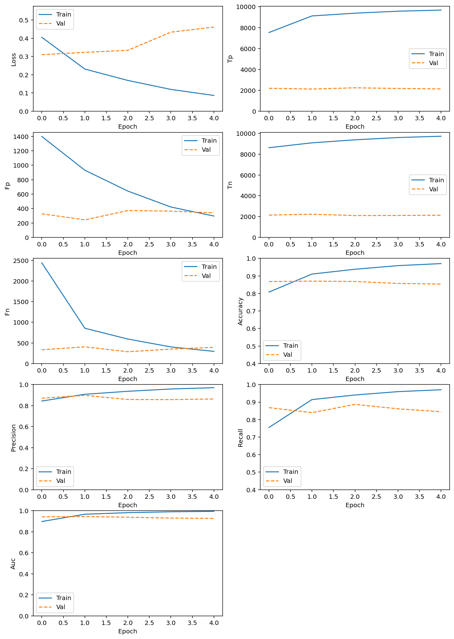
BATCH_SIZE = 100
EPOCHS = 5
history = model.fit(X_train,y_train,
                    batch_size=BATCH_SIZE,
                    epochs=EPOCHS,
                    validation_split=0.2)
Epoch 1/5
200/200 [==============================] - 48s 239ms/step - loss: 0.4054 - tp: 7530.0000 - fp: 1399.0000 - tn: 8629.0000 - fn: 2442.0000 - accuracy: 0.8080 - precision: 0.8433 - recall: 0.7551 - auc: 0.8971 - val_loss: 0.3101 - val_tp: 2195.0000 - val_fp: 327.0000 - val_tn: 2145.0000 - val_fn: 333.0000 - val_accuracy: 0.8680 - val_precision: 0.8703 - val_recall: 0.8683 - val_auc: 0.9415
Epoch 2/5
200/200 [==============================] - 45s 223ms/step - loss: 0.2312 - tp: 9116.0000 - fp: 931.0000 - tn: 9097.0000 - fn: 856.0000 - accuracy: 0.9107 - precision: 0.9073 - recall: 0.9142 - auc: 0.9665 - val_loss: 0.3227 - val_tp: 2123.0000 - val_fp: 243.0000 - val_tn: 2229.0000 - val_fn: 405.0000 - val_accuracy: 0.8704 - val_precision: 0.8973 - val_recall: 0.8398 - val_auc: 0.9444
Epoch 3/5
200/200 [==============================] - 43s 217ms/step - loss: 0.1689 - tp: 9378.0000 - fp: 642.0000 - tn: 9386.0000 - fn: 594.0000 - accuracy: 0.9382 - precision: 0.9359 - recall: 0.9404 - auc: 0.9814 - val_loss: 0.3340 - val_tp: 2242.0000 - val_fp: 372.0000 - val_tn: 2100.0000 - val_fn: 286.0000 - val_accuracy: 0.8684 - val_precision: 0.8577 - val_recall: 0.8869 - val_auc: 0.9382
Epoch 4/5
200/200 [==============================] - 45s 226ms/step - loss: 0.1197 - tp: 9569.0000 - fp: 421.0000 - tn: 9607.0000 - fn: 403.0000 - accuracy: 0.9588 - precision: 0.9579 - recall: 0.9596 - auc: 0.9897 - val_loss: 0.4335 - val_tp: 2178.0000 - val_fp: 364.0000 - val_tn: 2108.0000 - val_fn: 350.0000 - val_accuracy: 0.8572 - val_precision: 0.8568 - val_recall: 0.8616 - val_auc: 0.9298
Epoch 5/5
200/200 [==============================] - 45s 225ms/step - loss: 0.0866 - tp: 9677.0000 - fp: 296.0000 - tn: 9732.0000 - fn: 295.0000 - accuracy: 0.9704 - precision: 0.9703 - recall: 0.9704 - auc: 0.9940 - val_loss: 0.4615 - val_tp: 2136.0000 - val_fp: 340.0000 - val_tn: 2132.0000 - val_fn: 392.0000 - val_accuracy: 0.8536 - val_precision: 0.8627 - val_recall: 0.8449 - val_auc: 0.9268
# Loading the test dataset, and repeating the processing steps
df_test=pd.read_csv("../../../RepositoryData/data/IMDB/testData.tsv",header=0, delimiter="\t", quoting=3)
df_test.head()
df_test["review"]=df_test.review.apply(lambda x: clean_text(x))
df_test["sentiment"] = df_test["id"].map(lambda x: 1  if  int(x.strip('"').split("_")[1]) >= 5  else  0)
y_test = df_test["sentiment"]
list_sentences_test = df_test["review"]
list_tokenized_test = tokenizer.texts_to_sequences(list_sentences_test)
X_test = pad_sequences(list_tokenized_test, maxlen=MAX_LEN)

## Making predictions on our model
prediction = model.predict(X_test)
y_pred = (prediction > 0.5)
import numpy as np
import matplotlib as mpl
import matplotlib.pyplot as plt
import seaborn as sns
from sklearn.metrics import (classification_report,
                             confusion_matrix,
                             roc_auc_score)
%matplotlib inline
%config InlineBackend.figure_format = 'retina'

report = classification_report(y_test, y_pred)
print(report)

def plot_cm(labels, predictions, p=0.5):
    cm = confusion_matrix(labels, predictions)
    plt.figure(figsize=(5, 5))
    sns.heatmap(cm, annot=True, fmt="d")
    plt.title("Confusion matrix (non-normalized))")
    plt.ylabel("Actual label")
    plt.xlabel("Predicted label")

plot_cm(y_test, y_pred)
              precision    recall  f1-score   support

           0       0.83      0.87      0.85     12500
           1       0.86      0.83      0.84     12500

    accuracy                           0.85     25000
   macro avg       0.85      0.85      0.85     25000
weighted avg       0.85      0.85      0.85     25000

# Cross Validation Classification Accuracy

colors = plt.rcParams["axes.prop_cycle"].by_key()["color"]
mpl.rcParams["figure.figsize"] = (12, 18)

def plot_metrics(history):
    metrics = [
        "loss",
        "tp", "fp", "tn", "fn",
        "accuracy",
        "precision", "recall",
        "auc",
    ]
    for n, metric in  enumerate(metrics):
        name = metric.replace("_", " ").capitalize()
        plt.subplot(5, 2, n + 1)
        plt.plot(
            history.epoch,
            history.history[metric],
            color=colors[0],
            label="Train",
        )
        plt.plot(
            history.epoch,
            history.history["val_" + metric],
            color=colors[1],
            linestyle="--",
            label="Val",
        )
        plt.xlabel("Epoch")
        plt.ylabel(name)
        if metric == "loss":
            plt.ylim([0, plt.ylim()[1] * 1.2])
        elif metric == "accuracy":
            plt.ylim([0.4, 1])
        elif metric == "fn":
            plt.ylim([0, plt.ylim()[1]])
        elif metric == "fp":
            plt.ylim([0, plt.ylim()[1]])
        elif metric == "tn":
            plt.ylim([0, plt.ylim()[1]])
        elif metric == "tp":
            plt.ylim([0, plt.ylim()[1]])
        elif metric == "precision":
            plt.ylim([0, 1])
        elif metric == "recall":
            plt.ylim([0.4, 1])
        else:
            plt.ylim([0, 1])

        plt.legend()

plot_metrics(history)
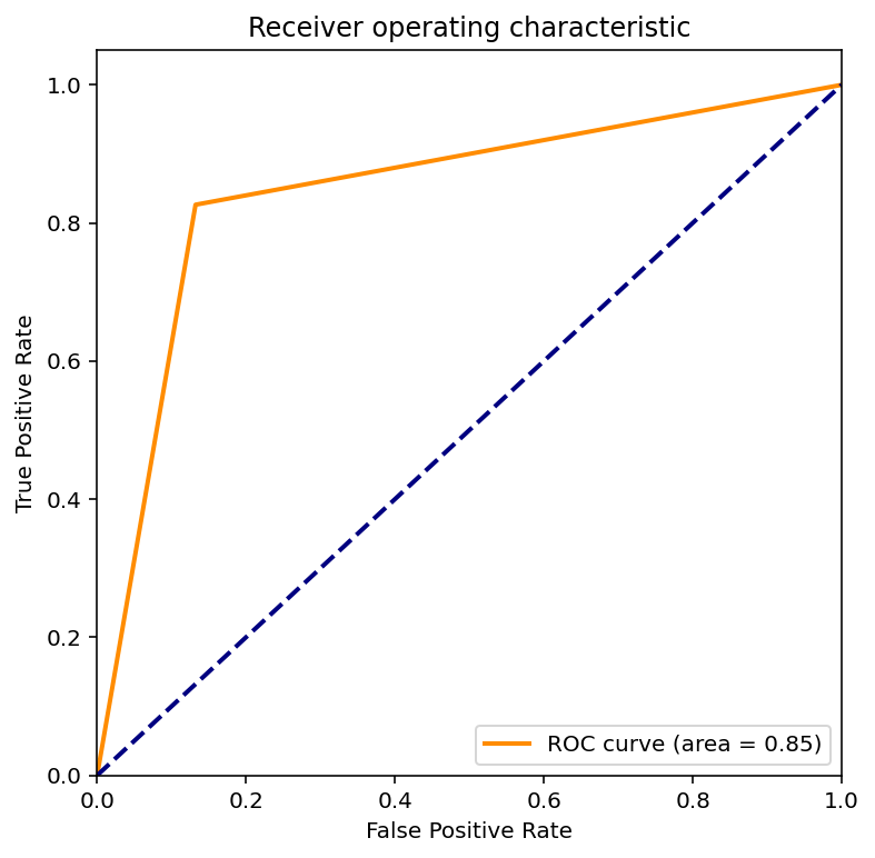
import numpy as np
import matplotlib.pyplot as plt
from itertools import cycle

mpl.rcParams["figure.figsize"] = (6, 6)

from sklearn import svm, datasets
from sklearn.metrics import roc_curve, auc
from sklearn.model_selection import train_test_split
from sklearn.preprocessing import label_binarize
from scipy import interp
from sklearn.metrics import roc_auc_score

# Binarize the output
y_bin = label_binarize(y_test, classes=[0, 1])
n_classes = 1

# Compute ROC curve and ROC area for each class
fpr = dict()
tpr = dict()
roc_auc = dict()
for i in  range(n_classes):
    fpr[i], tpr[i], _ = roc_curve(y_test.ravel(), y_pred.ravel())
    roc_auc[i] = auc(fpr[i], tpr[i])

# Compute micro-average ROC curve and ROC area
fpr["micro"], tpr["micro"], _ = roc_curve(y_test.ravel(), y_pred.ravel())
roc_auc["micro"] = auc(fpr["micro"], tpr["micro"])

plt.figure()
lw = 2
plt.plot(fpr[0], tpr[0], color='darkorange',
         lw=lw, label='ROC curve (area = %0.2f)' % roc_auc[0])
plt.plot([0, 1], [0, 1], color='navy', lw=lw, linestyle='--')
plt.xlim([0.0, 1.0])
plt.ylim([0.0, 1.05])
plt.xlabel('False Positive Rate')
plt.ylabel('True Positive Rate')
plt.title('Receiver operating characteristic')
plt.legend(loc="lower right")
plt.show()