
Sentiment Analysis Using Bag-of-Words#
Sentiment analysis is to analyze the textual documents and extract information that is related to the author’s sentiment or opinion. It is sometimes referred to as opinion mining.
It is popular and widely used in industry, e.g., corporate surveys, feedback surveys, social media data, reviews for movies, places, hotels, commodities, etc..
The sentiment information from texts can be crucial to further decision making in the industry.
Output of Sentiment Analysis
Qualitative: overall sentiment scale (positive/negative)
Quantitative: sentiment polarity scores
In this tutorial, we will use movie reviews as an example.
And the classification task is simple: to classify the document into one of the two classes, i.e., positive or negative.
Most importantly, we will be using mainly the module
sklearnfor creating and training the classifier.
import nltk, random
from nltk.corpus import movie_reviews
import pandas as pd
import matplotlib.pyplot as plt
import numpy as np
## Colab Only
nltk.download('movie_reviews')
!pip install lime textblob afinn
Data Loading#
We will use the corpus
nlkt.corpus.movie_reviewsas our data.Please download the corpus if you haven’t.
print(len(movie_reviews.fileids()))
print(movie_reviews.categories())
print(movie_reviews.words()[:100])
print(movie_reviews.fileids()[:10])
2000
['neg', 'pos']
['plot', ':', 'two', 'teen', 'couples', 'go', 'to', ...]
['neg/cv000_29416.txt', 'neg/cv001_19502.txt', 'neg/cv002_17424.txt', 'neg/cv003_12683.txt', 'neg/cv004_12641.txt', 'neg/cv005_29357.txt', 'neg/cv006_17022.txt', 'neg/cv007_4992.txt', 'neg/cv008_29326.txt', 'neg/cv009_29417.txt']
Rearrange the corpus data as a list of tuple, where the first element is the word tokens of the documents, and the second element is the label of the documents (i.e., sentiment labels).
documents = [(' '.join((movie_reviews.words(fileid))), category)
             for category in movie_reviews.categories()
             for fileid in movie_reviews.fileids(category)]

documents[:5]
[('plot : two teen couples go to a church party , drink and then drive . they get into an accident . one of the guys dies , but his girlfriend continues to see him in her life , and has nightmares . what \' s the deal ? watch the movie and " sorta " find out . . . critique : a mind - fuck movie for the teen generation that touches on a very cool idea , but presents it in a very bad package . which is what makes this review an even harder one to write , since i generally applaud films which attempt to break the mold , mess with your head and such ( lost highway & memento ) , but there are good and bad ways of making all types of films , and these folks just didn \' t snag this one correctly . they seem to have taken this pretty neat concept , but executed it terribly . so what are the problems with the movie ? well , its main problem is that it \' s simply too jumbled . it starts off " normal " but then downshifts into this " fantasy " world in which you , as an audience member , have no idea what \' s going on . there are dreams , there are characters coming back from the dead , there are others who look like the dead , there are strange apparitions , there are disappearances , there are a looooot of chase scenes , there are tons of weird things that happen , and most of it is simply not explained . now i personally don \' t mind trying to unravel a film every now and then , but when all it does is give me the same clue over and over again , i get kind of fed up after a while , which is this film \' s biggest problem . it \' s obviously got this big secret to hide , but it seems to want to hide it completely until its final five minutes . and do they make things entertaining , thrilling or even engaging , in the meantime ? not really . the sad part is that the arrow and i both dig on flicks like this , so we actually figured most of it out by the half - way point , so all of the strangeness after that did start to make a little bit of sense , but it still didn \' t the make the film all that more entertaining . i guess the bottom line with movies like this is that you should always make sure that the audience is " into it " even before they are given the secret password to enter your world of understanding . i mean , showing melissa sagemiller running away from visions for about 20 minutes throughout the movie is just plain lazy ! ! okay , we get it . . . there are people chasing her and we don \' t know who they are . do we really need to see it over and over again ? how about giving us different scenes offering further insight into all of the strangeness going down in the movie ? apparently , the studio took this film away from its director and chopped it up themselves , and it shows . there might \' ve been a pretty decent teen mind - fuck movie in here somewhere , but i guess " the suits " decided that turning it into a music video with little edge , would make more sense . the actors are pretty good for the most part , although wes bentley just seemed to be playing the exact same character that he did in american beauty , only in a new neighborhood . but my biggest kudos go out to sagemiller , who holds her own throughout the entire film , and actually has you feeling her character \' s unraveling . overall , the film doesn \' t stick because it doesn \' t entertain , it \' s confusing , it rarely excites and it feels pretty redundant for most of its runtime , despite a pretty cool ending and explanation to all of the craziness that came before it . oh , and by the way , this is not a horror or teen slasher flick . . . it \' s just packaged to look that way because someone is apparently assuming that the genre is still hot with the kids . it also wrapped production two years ago and has been sitting on the shelves ever since . whatever . . . skip it ! where \' s joblo coming from ? a nightmare of elm street 3 ( 7 / 10 ) - blair witch 2 ( 7 / 10 ) - the crow ( 9 / 10 ) - the crow : salvation ( 4 / 10 ) - lost highway ( 10 / 10 ) - memento ( 10 / 10 ) - the others ( 9 / 10 ) - stir of echoes ( 8 / 10 )',
  'neg'),
 ('the happy bastard \' s quick movie review damn that y2k bug . it \' s got a head start in this movie starring jamie lee curtis and another baldwin brother ( william this time ) in a story regarding a crew of a tugboat that comes across a deserted russian tech ship that has a strangeness to it when they kick the power back on . little do they know the power within . . . going for the gore and bringing on a few action sequences here and there , virus still feels very empty , like a movie going for all flash and no substance . we don \' t know why the crew was really out in the middle of nowhere , we don \' t know the origin of what took over the ship ( just that a big pink flashy thing hit the mir ) , and , of course , we don \' t know why donald sutherland is stumbling around drunkenly throughout . here , it \' s just " hey , let \' s chase these people around with some robots " . the acting is below average , even from the likes of curtis . you \' re more likely to get a kick out of her work in halloween h20 . sutherland is wasted and baldwin , well , he \' s acting like a baldwin , of course . the real star here are stan winston \' s robot design , some schnazzy cgi , and the occasional good gore shot , like picking into someone \' s brain . so , if robots and body parts really turn you on , here \' s your movie . otherwise , it \' s pretty much a sunken ship of a movie .',
  'neg'),
 ("it is movies like these that make a jaded movie viewer thankful for the invention of the timex indiglo watch . based on the late 1960 ' s television show by the same name , the mod squad tells the tale of three reformed criminals under the employ of the police to go undercover . however , things go wrong as evidence gets stolen and they are immediately under suspicion . of course , the ads make it seem like so much more . quick cuts , cool music , claire dane ' s nice hair and cute outfits , car chases , stuff blowing up , and the like . sounds like a cool movie , does it not ? after the first fifteen minutes , it quickly becomes apparent that it is not . the mod squad is certainly a slick looking production , complete with nice hair and costumes , but that simply isn ' t enough . the film is best described as a cross between an hour - long cop show and a music video , both stretched out into the span of an hour and a half . and with it comes every single clich ? . it doesn ' t really matter that the film is based on a television show , as most of the plot elements have been recycled from everything we ' ve already seen . the characters and acting is nothing spectacular , sometimes even bordering on wooden . claire danes and omar epps deliver their lines as if they are bored , which really transfers onto the audience . the only one to escape relatively unscathed is giovanni ribisi , who plays the resident crazy man , ultimately being the only thing worth watching . unfortunately , even he ' s not enough to save this convoluted mess , as all the characters don ' t do much apart from occupying screen time . with the young cast , cool clothes , nice hair , and hip soundtrack , it appears that the film is geared towards the teenage mindset . despite an american ' r ' rating ( which the content does not justify ) , the film is way too juvenile for the older mindset . information on the characters is literally spoon - fed to the audience ( would it be that hard to show us instead of telling us ? ) , dialogue is poorly written , and the plot is extremely predictable . the way the film progresses , you likely won ' t even care if the heroes are in any jeopardy , because you ' ll know they aren ' t . basing the show on a 1960 ' s television show that nobody remembers is of questionable wisdom , especially when one considers the target audience and the fact that the number of memorable films based on television shows can be counted on one hand ( even one that ' s missing a finger or two ) . the number of times that i checked my watch ( six ) is a clear indication that this film is not one of them . it is clear that the film is nothing more than an attempt to cash in on the teenage spending dollar , judging from the rash of really awful teen - flicks that we ' ve been seeing as of late . avoid this film at all costs .",
  'neg'),
 ('" quest for camelot " is warner bros . \' first feature - length , fully - animated attempt to steal clout from disney \' s cartoon empire , but the mouse has no reason to be worried . the only other recent challenger to their throne was last fall \' s promising , if flawed , 20th century fox production " anastasia , " but disney \' s " hercules , " with its lively cast and colorful palate , had her beat hands - down when it came time to crown 1997 \' s best piece of animation . this year , it \' s no contest , as " quest for camelot " is pretty much dead on arrival . even the magic kingdom at its most mediocre -- that \' d be " pocahontas " for those of you keeping score -- isn \' t nearly as dull as this . the story revolves around the adventures of free - spirited kayley ( voiced by jessalyn gilsig ) , the early - teen daughter of a belated knight from king arthur \' s round table . kayley \' s only dream is to follow in her father \' s footsteps , and she gets her chance when evil warlord ruber ( gary oldman ) , an ex - round table member - gone - bad , steals arthur \' s magical sword excalibur and accidentally loses it in a dangerous , booby - trapped forest . with the help of hunky , blind timberland - dweller garrett ( carey elwes ) and a two - headed dragon ( eric idle and don rickles ) that \' s always arguing with itself , kayley just might be able to break the medieval sexist mold and prove her worth as a fighter on arthur \' s side . " quest for camelot " is missing pure showmanship , an essential element if it \' s ever expected to climb to the high ranks of disney . there \' s nothing here that differentiates " quest " from something you \' d see on any given saturday morning cartoon -- subpar animation , instantly forgettable songs , poorly - integrated computerized footage . ( compare kayley and garrett \' s run - in with the angry ogre to herc \' s battle with the hydra . i rest my case . ) even the characters stink -- none of them are remotely interesting , so much that the film becomes a race to see which one can out - bland the others . in the end , it \' s a tie -- they all win . that dragon \' s comedy shtick is awfully cloying , but at least it shows signs of a pulse . at least fans of the early -\' 90s tgif television line - up will be thrilled to find jaleel " urkel " white and bronson " balki " pinchot sharing the same footage . a few scenes are nicely realized ( though i \' m at a loss to recall enough to be specific ) , and the actors providing the voice talent are enthusiastic ( though most are paired up with singers who don \' t sound a thing like them for their big musical moments -- jane seymour and celine dion ? ? ? ) . but one must strain through too much of this mess to find the good . aside from the fact that children will probably be as bored watching this as adults , " quest for camelot " \' s most grievous error is its complete lack of personality . and personality , we learn from this mess , goes a very long way .',
  'neg'),
 ('synopsis : a mentally unstable man undergoing psychotherapy saves a boy from a potentially fatal accident and then falls in love with the boy \' s mother , a fledgling restauranteur . unsuccessfully attempting to gain the woman \' s favor , he takes pictures of her and kills a number of people in his way . comments : stalked is yet another in a seemingly endless string of spurned - psychos - getting - their - revenge type movies which are a stable category in the 1990s film industry , both theatrical and direct - to - video . their proliferation may be due in part to the fact that they \' re typically inexpensive to produce ( no special effects , no big name stars ) and serve as vehicles to flash nudity ( allowing them to frequent late - night cable television ) . stalked wavers slightly from the norm in one respect : the psycho never actually has an affair ; on the contrary , he \' s rejected rather quickly ( the psycho typically is an ex - lover , ex - wife , or ex - husband ) . other than that , stalked is just another redundant entry doomed to collect dust on video shelves and viewed after midnight on cable . stalked does not provide much suspense , though that is what it sets out to do . interspersed throughout the opening credits , for instance , a serious - sounding narrator spouts statistics about stalkers and ponders what may cause a man to stalk ( it \' s implicitly implied that all stalkers are men ) while pictures of a boy are shown on the screen . after these credits , a snapshot of actor jay underwood appears . the narrator states that " this is the story of daryl gleason " and tells the audience that he is the stalker . of course , really , this is the story of restauranteur brooke daniels . if the movie was meant to be about daryl , then it should have been called stalker not stalked . okay . so we know who the stalker is even before the movie starts ; no guesswork required . stalked proceeds , then , as it begins : obvious , obvious , obvious . the opening sequence , contrived quite a bit , brings daryl and brooke ( the victim ) together . daryl obsesses over brooke , follows her around , and tries to woo her . ultimately rejected by her , his plans become more and more desperate and elaborate . these plans include the all - time , psycho - in - love , cliche : the murdered pet . for some reason , this genre \' s films require a dead pet to be found by the victim stalked . stalked is no exception ( it \' s a cat this time -- found in the shower ) . events like these lead to the inevitable showdown between stalker and stalked , where only one survives ( guess who it invariably always is and you \' ll guess the conclusion to this turkey ) . stalked \' s cast is uniformly adequate : not anything to write home about but also not all that bad either . jay underwood , as the stalker , turns toward melodrama a bit too much . he overdoes it , in other words , but he still manages to be creepy enough to pass as the type of stalker the story demands . maryam d \' abo , about the only actor close to being a star here ( she played the bond chick in the living daylights ) , is equally adequate as the " stalked " of the title , even though she seems too ditzy at times to be a strong , independent business - owner . brooke ( d \' abo ) needs to be ditzy , however , for the plot to proceed . toward the end , for example , brooke has her suspicions about daryl . to ensure he won \' t use it as another excuse to see her , brooke decides to return a toolbox he had left at her place to his house . does she just leave the toolbox at the door when no one answers ? of course not . she tries the door , opens it , and wanders around the house . when daryl returns , he enters the house , of course , so our heroine is in danger . somehow , even though her car is parked at the front of the house , right by the front door , daryl is oblivious to her presence inside . the whole episode places an incredible strain on the audience \' s suspension of disbelief and questions the validity of either character \' s intelligence . stalked receives two stars because , even though it is highly derivative and somewhat boring , it is not so bad that it cannot be watched . rated r mostly for several murder scenes and brief nudity in a strip bar , it is not as offensive as many other thrillers in this genre are . if you \' re in the mood for a good suspense film , though , stake out something else .',
  'neg')]
Corpus Profile#
Important descriptive statistics:
Corpus Size (Number of Documents)
Corpus Size (Number of Words)
Distribution of the Two Classes
It is important to always report the above necessary descriptive statistics when presenting your classifiers.
print('Number of Reviews/Documents: {}'.format(len(documents)))
print('Corpus Size (words): {}'.format(np.sum([len(d) for (d,l) in documents])))
print('Max Doc Size (words): {}'.format(np.max([len(d) for (d,l) in documents])))
print('Min Doc Size (words): {}'.format(np.min([len(d) for (d,l) in documents])))
print('Average Doc Size (words): {}'.format(np.mean([len(d) for (d,l) in documents])))
print('Sample Text of Doc 1:')
print('-'*30)
print(' '.join(documents[0][:50])) # first 50 words of the first document
Number of Reviews/Documents: 2000
Corpus Size (words): 7808520
Max Doc Size (words): 15097
Min Doc Size (words): 91
Average Doc Size (words): 3904.26
Sample Text of Doc 1:
------------------------------
plot : two teen couples go to a church party , drink and then drive . they get into an accident . one of the guys dies , but his girlfriend continues to see him in her life , and has nightmares . what ' s the deal ? watch the movie and " sorta " find out . . . critique : a mind - fuck movie for the teen generation that touches on a very cool idea , but presents it in a very bad package . which is what makes this review an even harder one to write , since i generally applaud films which attempt to break the mold , mess with your head and such ( lost highway & memento ) , but there are good and bad ways of making all types of films , and these folks just didn ' t snag this one correctly . they seem to have taken this pretty neat concept , but executed it terribly . so what are the problems with the movie ? well , its main problem is that it ' s simply too jumbled . it starts off " normal " but then downshifts into this " fantasy " world in which you , as an audience member , have no idea what ' s going on . there are dreams , there are characters coming back from the dead , there are others who look like the dead , there are strange apparitions , there are disappearances , there are a looooot of chase scenes , there are tons of weird things that happen , and most of it is simply not explained . now i personally don ' t mind trying to unravel a film every now and then , but when all it does is give me the same clue over and over again , i get kind of fed up after a while , which is this film ' s biggest problem . it ' s obviously got this big secret to hide , but it seems to want to hide it completely until its final five minutes . and do they make things entertaining , thrilling or even engaging , in the meantime ? not really . the sad part is that the arrow and i both dig on flicks like this , so we actually figured most of it out by the half - way point , so all of the strangeness after that did start to make a little bit of sense , but it still didn ' t the make the film all that more entertaining . i guess the bottom line with movies like this is that you should always make sure that the audience is " into it " even before they are given the secret password to enter your world of understanding . i mean , showing melissa sagemiller running away from visions for about 20 minutes throughout the movie is just plain lazy ! ! okay , we get it . . . there are people chasing her and we don ' t know who they are . do we really need to see it over and over again ? how about giving us different scenes offering further insight into all of the strangeness going down in the movie ? apparently , the studio took this film away from its director and chopped it up themselves , and it shows . there might ' ve been a pretty decent teen mind - fuck movie in here somewhere , but i guess " the suits " decided that turning it into a music video with little edge , would make more sense . the actors are pretty good for the most part , although wes bentley just seemed to be playing the exact same character that he did in american beauty , only in a new neighborhood . but my biggest kudos go out to sagemiller , who holds her own throughout the entire film , and actually has you feeling her character ' s unraveling . overall , the film doesn ' t stick because it doesn ' t entertain , it ' s confusing , it rarely excites and it feels pretty redundant for most of its runtime , despite a pretty cool ending and explanation to all of the craziness that came before it . oh , and by the way , this is not a horror or teen slasher flick . . . it ' s just packaged to look that way because someone is apparently assuming that the genre is still hot with the kids . it also wrapped production two years ago and has been sitting on the shelves ever since . whatever . . . skip it ! where ' s joblo coming from ? a nightmare of elm street 3 ( 7 / 10 ) - blair witch 2 ( 7 / 10 ) - the crow ( 9 / 10 ) - the crow : salvation ( 4 / 10 ) - lost highway ( 10 / 10 ) - memento ( 10 / 10 ) - the others ( 9 / 10 ) - stir of echoes ( 8 / 10 ) neg
## Check Sentiment Distribution of the Current Dataset
from collections import Counter
sentiment_distr = Counter([label for (words, label) in documents])
print(sentiment_distr)
Counter({'neg': 1000, 'pos': 1000})
Random Shuffle#
Shuffling the training data randomizes the order in which samples are presented to the model during training. This prevents the model from learning any patterns or sequences in the data that might not generalize well to unseen data.
Shuffling helps prevent the model from memorizing the order of samples, ensuring it focuses on learning the underlying patterns in the data.
It improves the generalizability of the model by reducing the risk of overfitting to specific patterns in the training data.
Shuffling is particularly important when dealing with imbalanced datasets, as it ensures that each batch or epoch contains a representative sample of the entire dataset [4].
import random

random.seed(123)
random.shuffle(documents)
Note
Specifying a random seed in Python is essential for ensuring reproducibility in random processes. By setting a seed value before generating random numbers, it initializes the pseudo-random number generator to produce the same sequence of random values each time the code is executed with the same seed, thus guaranteeing consistent results across different runs. This is particularly useful in situations where you need deterministic behavior, such as debugging, testing, or ensuring consistent model training outcomes in machine learning
Data Preprocessing#
Depending on our raw data, we may need data preprocessing before feature engineering so as to remove irrelevant information from our data.
In this example, bag-of-word methods require very little preprocessing.
Train-Test Split#
We split the entire dataset into two parts: training set and testing set.
The proportion of training and testing sets may depend on the corpus size.
In the train-test split, make sure the the distribution of the classes is proportional.
from sklearn.model_selection import train_test_split
train, test = train_test_split(documents, test_size = 0.33, random_state=42)
## Sentiment Distrubtion for Train and Test
print(Counter([label for (text, label) in train]))
print(Counter([label for (text, label) in test]))
Counter({'neg': 674, 'pos': 666})
Counter({'pos': 334, 'neg': 326})
Because in most of the ML steps, the feature sets and the labels are often separated as two units, we split our training data into
X_trainandy_trainas the features (X) and labels (y) in training.Likewise, we split our testing data into
X_testandy_testas the features (X) and labels (y) in testing.
X_train = [text for (text, label) in train]
X_test = [text for (text, label) in test]
y_train = [label for (text, label) in train]
y_test = [label for (text, label) in test]
Text Vectorization#
In feature-based machine learning, we need to vectorize texts into feature sets (i.e., feature engineering on texts).
We use the naive bag-of-words text vectorization. In particular, we use the weighted version of BOW.
from sklearn.feature_extraction.text import CountVectorizer, TfidfVectorizer

tfidf_vec = TfidfVectorizer(min_df = 10, token_pattern = r'[a-zA-Z]+')
X_train_bow = tfidf_vec.fit_transform(X_train) # fit train
X_test_bow = tfidf_vec.transform(X_test) # transform test
Important Notes:
Always split the data into train and test first before vectorizing the texts
Otherwise, you would leak information to the training process, which may lead to over-fitting
When vectorizing the texts,
fit_transform()on the training set andtransform()on the testing set.Always report the number of features used in the model.
print(X_train_bow.shape)
print(X_test_bow.shape)
(1340, 6138)
(660, 6138)
Model Selection and Cross Validation#
For our current binary sentiment classifier, we will try a few common classification algorithms:
Support Vector Machine
Decision Tree
Naive Bayes
Logistic Regression
The common steps include:
We fit the model with our training data.
We check the model stability, using k-fold cross validation on the training data.
We use the fitted model to make prediction.
We evaluate the model prediction by comparing the predicted classes and the true labels.
SVM#
from sklearn import svm

model_svm = svm.SVC(C=8.0, kernel='linear')
model_svm.fit(X_train_bow, y_train)
SVC(C=8.0, kernel='linear')In a Jupyter environment, please rerun this cell to show the HTML representation or trust the notebook.
On GitHub, the HTML representation is unable to render, please try loading this page with nbviewer.org.
SVC(C=8.0, kernel='linear')
from sklearn.model_selection import cross_val_score
model_svm_acc = cross_val_score(estimator=model_svm, X=X_train_bow, y=y_train, cv=5, n_jobs=-1)
model_svm_acc
array([0.84328358, 0.82089552, 0.85447761, 0.82462687, 0.84701493])
model_svm.predict(X_test_bow[:10])
#print(model_svm.score(test_text_bow, test_label))
array(['pos', 'neg', 'pos', 'neg', 'neg', 'neg', 'neg', 'neg', 'neg',
       'pos'], dtype='<U3')
Decision Tree#
from sklearn.tree import DecisionTreeClassifier

model_dec = DecisionTreeClassifier(max_depth=10, random_state=0)
model_dec.fit(X_train_bow, y_train)
DecisionTreeClassifier(max_depth=10, random_state=0)In a Jupyter environment, please rerun this cell to show the HTML representation or trust the notebook.
On GitHub, the HTML representation is unable to render, please try loading this page with nbviewer.org.
DecisionTreeClassifier(max_depth=10, random_state=0)
model_dec_acc = cross_val_score(estimator=model_dec, X=X_train_bow, y=y_train, cv=5, n_jobs=-1)
model_dec_acc
array([0.6641791 , 0.64179104, 0.66791045, 0.64179104, 0.6380597 ])
model_dec.predict(X_test_bow[:10])
array(['pos', 'neg', 'neg', 'neg', 'pos', 'pos', 'neg', 'neg', 'neg',
       'neg'], dtype='<U3')
Naive Bayes#
from sklearn.naive_bayes import GaussianNB
model_gnb = GaussianNB()
model_gnb.fit(X_train_bow.toarray(), y_train)
GaussianNB()In a Jupyter environment, please rerun this cell to show the HTML representation or trust the notebook.
On GitHub, the HTML representation is unable to render, please try loading this page with nbviewer.org.
GaussianNB()
model_gnb_acc = cross_val_score(estimator=model_gnb, X=X_train_bow.toarray(), y=y_train, cv=5, n_jobs=-1)
model_gnb_acc
array([0.7238806 , 0.67164179, 0.7238806 , 0.68656716, 0.68283582])
model_gnb.predict(X_test_bow[:10].toarray())
array(['pos', 'neg', 'neg', 'neg', 'neg', 'neg', 'neg', 'neg', 'neg',
       'neg'], dtype='<U3')
Logistic Regression#
from sklearn.linear_model import LogisticRegression

model_lg = LogisticRegression()
model_lg.fit(X_train_bow, y_train)
LogisticRegression()In a Jupyter environment, please rerun this cell to show the HTML representation or trust the notebook.
On GitHub, the HTML representation is unable to render, please try loading this page with nbviewer.org.
LogisticRegression()
model_lg_acc = cross_val_score(estimator=model_lg, X=X_train_bow, y=y_train, cv=5, n_jobs=-1)
model_lg_acc
array([0.83208955, 0.79477612, 0.82462687, 0.78731343, 0.82835821])
model_lg.predict(X_test_bow[:10].toarray())
array(['pos', 'neg', 'pos', 'neg', 'neg', 'pos', 'neg', 'neg', 'neg',
       'pos'], dtype='<U3')
Cross Validation (LR as an example)#
Cross-validation is a technique used in machine learning to assess how well a predictive model will perform on unseen data.
By dividing the dataset into multiple subsets, it trains the model on a portion of the data and evaluates it on the remaining data.
This process is repeated several times, with each subset serving as both training and validation data.
Benefits of Cross-validation:
provides more reliable estimates of model performanc
reduces overfitting by testing the model on different data subsets
maximizes data utilization
facilitates hyperparameter tuning
assesses the model’s generalization ability (biases vs. variation)
from sklearn.model_selection import cross_val_score

# Perform cross-validation
scores = cross_val_score(model_lg,          ## base model
                         X_train_bow,       ## X
                         y_train,           ## y
                         cv=10)             ## 10-fold cross-validation

# Print scores
print(scores)
print("Average Score:", scores.mean())
[0.82089552 0.82089552 0.79104478 0.80597015 0.85074627 0.82835821
 0.80597015 0.79850746 0.82835821 0.8358209 ]
Average Score: 0.8186567164179104
You can perform cross-validation using the other classifiers to see which machine learning algorithm gives you the more stable predictions on the training set.
Evaluation#
To evaluate each model’s performance, there are several common metrics in use:
Precision
Recall
F-score
Accuracy
Confusion Matrix
#Mean Accuracy
print(model_svm.score(X_test_bow, y_test))
print(model_dec.score(X_test_bow, y_test))
print(model_gnb.score(X_test_bow.toarray(), y_test))
print(model_lg.score(X_test_bow, y_test))
0.8075757575757576
0.65
0.7015151515151515
0.7954545454545454
# F1
from sklearn.metrics import f1_score

y_pred = model_svm.predict(X_test_bow)

f1_score(y_test, y_pred,
         average=None,
         labels = movie_reviews.categories())
array([0.80248834, 0.81240768])
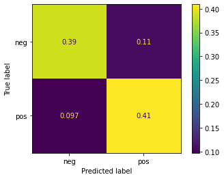
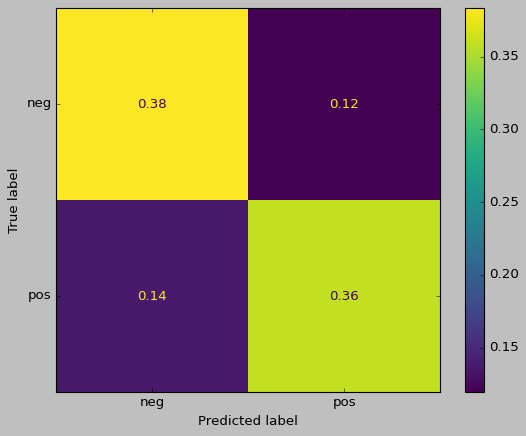
from sklearn.metrics import ConfusionMatrixDisplay

ConfusionMatrixDisplay.from_estimator(model_svm, X_test_bow, y_test, normalize='all')
<sklearn.metrics._plot.confusion_matrix.ConfusionMatrixDisplay at 0x1118b72b0>

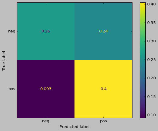
ConfusionMatrixDisplay.from_estimator(model_lg, X_test_bow.toarray(), y_test, normalize='all')
<sklearn.metrics._plot.confusion_matrix.ConfusionMatrixDisplay at 0x2b7e00220>
## try a whole new self-created review:)
new_review =['This book looks soso like the content but the cover is weird',
             'This book looks soso like the content and the cover is weird'
            ]
new_review_bow = tfidf_vec.transform(new_review)
model_svm.predict(new_review_bow)
array(['neg', 'neg'], dtype='<U3')
Tuning Model Hyperparameters - Grid Search#
For each model, we have not optimized it in terms of its hyperparameter setting.
Now that SVM seems to perform the best among all, we take this as our base model and further fine-tune its hyperparameter using cross-validation and Grid Search.
%%time

from sklearn.model_selection import GridSearchCV

parameters = {'kernel': ('linear', 'rbf'), 'C': (1,4,8,16,32)}

svc = svm.SVC()
clf = GridSearchCV(svc, parameters, cv=10, n_jobs=-1) ## `-1` run in parallel
clf.fit(X_train_bow, y_train)
/Users/alvinchen/anaconda3/envs/python-notes/lib/python3.9/site-packages/joblib/externals/loky/process_executor.py:752: UserWarning: A worker stopped while some jobs were given to the executor. This can be caused by a too short worker timeout or by a memory leak.
  warnings.warn(
CPU times: user 2.14 s, sys: 71.8 ms, total: 2.21 s
Wall time: 26.3 s
GridSearchCV(cv=10, estimator=SVC(), n_jobs=-1,
             param_grid={'C': (1, 4, 8, 16, 32), 'kernel': ('linear', 'rbf')})
In a Jupyter environment, please rerun this cell to show the HTML representation or trust the notebook. On GitHub, the HTML representation is unable to render, please try loading this page with nbviewer.org.
GridSearchCV(cv=10, estimator=SVC(), n_jobs=-1,
param_grid={'C': (1, 4, 8, 16, 32), 'kernel': ('linear', 'rbf')})SVC()
SVC()
We can check the parameters that yield the most optimal results in the Grid Search:
#print(sorted(clf.cv_results_.keys()))
print(clf.best_params_)
{'C': 1, 'kernel': 'linear'}
print(clf.score(X_test_bow, y_test))
0.8106060606060606
Post-hoc Analysis#
After we find the optimal classifier, next comes the most important step: interpret the classifier.
A good classifier may not always perform as we have expected. Chances are that the classifier may have used cues that are unexpected for decision making.
In the post-hoc analysis, we are interested in:
Which features contribute to the classifier’s prediction the most?
Which features are more relevant to each class prediction?
We will introduce three methods for post-hoc analysis:
LIME
Model coefficients and feature importance
Permutation importances
LIME#
Using LIME (Local Interpretable Model-agnostic Explanations) to interpret the importance of the features in relation to the model prediction.
LIME was introduced in 2016 by Marco Ribeiro and his collaborators in a paper called “Why Should I Trust You?” Explaining the Predictions of Any Classifier
Its objective is to explain a model prediction for a specific text sample in a human-interpretable way.
What we have done so far tells us that the model accuracy is good, but we have no idea whether the classifier has learned features that are useful and meaningful.
How can we identify important words that may have great contribution to the model prediction?
import lime
from lime.lime_text import LimeTextExplainer
from sklearn.pipeline import Pipeline
## define the pipeline
pipeline = Pipeline([
  ('vectorizer',tfidf_vec),
  ('clf', svm.SVC(C=1, kernel='linear', probability=True))])

## Refit model based on optimal parameter settings
pipeline.fit(X_train, y_train)
Pipeline(steps=[('vectorizer',
                 TfidfVectorizer(min_df=10, token_pattern='[a-zA-Z]+')),
                ('clf', SVC(C=1, kernel='linear', probability=True))])
In a Jupyter environment, please rerun this cell to show the HTML representation or trust the notebook. On GitHub, the HTML representation is unable to render, please try loading this page with nbviewer.org.
Pipeline(steps=[('vectorizer',
                 TfidfVectorizer(min_df=10, token_pattern='[a-zA-Z]+')),
('clf', SVC(C=1, kernel='linear', probability=True))])TfidfVectorizer(min_df=10, token_pattern='[a-zA-Z]+')
SVC(C=1, kernel='linear', probability=True)
import textwrap
reviews_test = X_test
sentiments_test = y_test


# We choose a sample from test set
idx = 210
text_sample = reviews_test[idx]
class_names = ['negative', 'positive']

print('Review ID-{}:'.format(idx))
print('-'*50)
print('Review Text:\n', textwrap.fill(text_sample,400))
print('-'*50)
print('Probability(positive) =', pipeline.predict_proba([text_sample])[0,1])
print('Probability(negative) =', pipeline.predict_proba([text_sample])[0,0])
print('Predicted class: %s' % pipeline.predict([text_sample]))
print('True class: %s' % sentiments_test[idx])
Review ID-210:
--------------------------------------------------
Review Text:
 in ` enemy at the gates ' , jude law is a gifted russian sniper made hero by a political officer named danilov ( joseph fiennes ) who uses him in a propaganda newspaper to raise the hopes of the soldiers and people of stalingrad . it ' s world war ii , and the russian - german standoff in town could determine the outcome of things for the motherland . law ' s vassili is the russian ' s top pawn to
victory . lots of war stuff happens . an older , german version of jude ' s character played by ed harris shows up halfway into the proceedings . he ' s equally talented , and the two men play a cat and mouse game trying to kill each other . they constantly switch roles , as the war fades far into the background . the cast also includes the terrific rachel weisz as a love interest for both vassili
and danilov the set - up is decent , and so are the production values . boasting a wide range of grimy locales , greasy hair , and tattered costumes , the art direction prospers . the actors , however , suffer the problem matt damon had in ` saving private ryan ' . either their eyes , teeth , skin , or a combination of other features looked too white and clean . with dirt and blood all around ,
the blinding teeth or bright eyes of these actors divert attention from the action . that said , the players are mostly good in their roles , although i don ' t think ed harris was really trying . maybe he realized his role struck a difficult chord in one - notedom . while the film is technically about snipers , there are far too many predictable sniping scenes . director jean - jacques annaud
expects us to view each tense situation with jude and some cohort in a tight spot as edgy and exciting , but after about the sixth time , in which we realize that jude is not going to die , it ' s relatively pointless . we get that he ' s talented , okay , let ' s move on . that ' s the problem with ` enemy at the gates ' ; it just doesn ' t know when to stop . witness the wasted seventeen minutes
that could have been spent elsewhere . reestablishing his title as the most beautiful ( and often talented ) man on film , jude law carries the movie . without him , this costly production would have gone into the ground . the story and acting are of good quality , but there ' s never a sense of authenticity or reality . something about this war movie is undeniably modern , and it loses its
feeling . strange enough , the screenplay is based on the true story of a real russian sniper .
--------------------------------------------------
Probability(positive) = 0.7430335079615914
Probability(negative) = 0.25696649203840877
Predicted class: ['pos']
True class: pos
import matplotlib
matplotlib.rcParams['figure.dpi']=300
%matplotlib inline


explainer = LimeTextExplainer(class_names=class_names)
explanation = explainer.explain_instance(text_sample,
                                         pipeline.predict_proba,
                                         num_features=20)
explanation.show_in_notebook(text=True)
Model Coefficients and Feature Importance#
Another way to evaluate the importance of the features is to look at their corresponding coefficients.
Positive weights imply positive contribution of the feature to the prediction; negative weights imply negative contribution of the feature to the prediction.
The absolute values of the weights indicate the effect sizes of the features.
Not all ML models provide “coefficients”.
## Extract the coefficients of the model from the pipeline
importances = pipeline.named_steps['clf'].coef_.toarray().flatten()
## Select top 10 positive/negative weights
top_indices_pos = np.argsort(importances)[::-1][:10]
top_indices_neg = np.argsort(importances)[:10]
## Get featnames from tfidfvectorizer
feature_names = np.array(tfidf_vec.get_feature_names_out()) # List indexing is different from array
feature_importance_df = pd.DataFrame({'FEATURE': feature_names[np.concatenate((top_indices_pos, top_indices_neg))],
                                     'IMPORTANCE': importances[np.concatenate((top_indices_pos, top_indices_neg))],
                                     'SENTIMENT': ['pos' for _ in range(len(top_indices_pos))]+['neg' for _ in range(len(top_indices_neg))]})
feature_importance_df
| FEATURE | IMPORTANCE | SENTIMENT | |
|---|---|---|---|
| 0 | and | 2.718226 | pos |
| 1 | fun | 1.582112 | pos |
| 2 | rocky | 1.577557 | pos |
| 3 | well | 1.555922 | pos |
| 4 | great | 1.486346 | pos |
| 5 | also | 1.441834 | pos |
| 6 | you | 1.385660 | pos |
| 7 | hilarious | 1.382671 | pos |
| 8 | mulan | 1.361607 | pos |
| 9 | life | 1.343015 | pos |
| 10 | bad | -2.942730 | neg |
| 11 | plot | -1.982912 | neg |
| 12 | have | -1.949701 | neg |
| 13 | even | -1.793556 | neg |
| 14 | boring | -1.721138 | neg |
| 15 | worst | -1.675429 | neg |
| 16 | there | -1.589407 | neg |
| 17 | nothing | -1.543166 | neg |
| 18 | only | -1.514030 | neg |
| 19 | why | -1.442169 | neg |
import pandas as pd
import matplotlib.pyplot as plt
import seaborn as sns
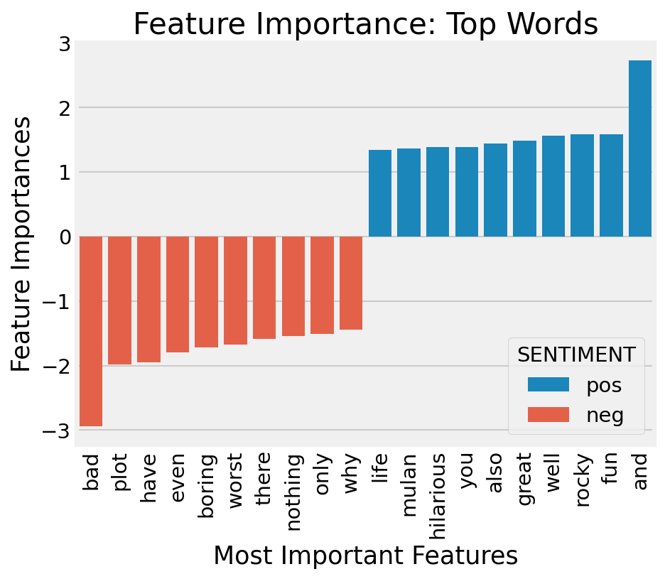
## Barplot (sorted by importance values)
plt.figure(figsize=(7,5), dpi=150)
plt.style.use('fivethirtyeight')
# print(plt.style.available)
# plt.bar(x = feature_importance_df['FEATURE'], height=feature_importance_df['IMPORTANCE'])
sns.barplot(x = 'FEATURE', y = 'IMPORTANCE', data = feature_importance_df,
hue = 'SENTIMENT', dodge = False,
order = feature_importance_df.sort_values('IMPORTANCE').FEATURE)
plt.xlabel("Most Important Features")
plt.ylabel("Feature Importances")
plt.xticks(rotation=90)
plt.title("Feature Importance: Top Words", color="black")
Text(0.5, 1.0, 'Feature Importance: Top Words')
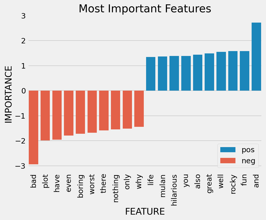
## Barplot sorted by importance values (II)

# Reorder the features based on their importance
feature_importance_df['FEATURE'] = pd.Categorical(feature_importance_df['FEATURE'], ordered=True, categories=feature_importance_df.sort_values('IMPORTANCE')['FEATURE'])

# Create the bar plot
plt.figure(figsize= (7, 5),dpi=150)
sns.barplot(x='FEATURE', y='IMPORTANCE', hue='SENTIMENT', data=feature_importance_df, dodge=False)
plt.title('Most Important Features')
plt.xlabel('FEATURE')
plt.ylabel('IMPORTANCE')
plt.legend(title=None)
plt.xticks(rotation=90)
plt.show()
Permutation Importances#
Permutation importances measure the impact of shuffling a single feature’s values on the model’s performance. It quantifies how much the model relies on each feature for making predictions.
The permutation importance is computed as the decrease in the model’s performance (e.g., accuracy) when the values of a particular feature are randomly shuffled. The larger the decrease in performance, the more important the feature is considered to be.
Positive permutation importance indicates that shuffling the feature leads to a significant drop in model performance, suggesting higher importance of that feature.
Negative permutation importance suggests that shuffling the feature has little impact on model performance, indicating lower importance or redundancy of that feature.
See
sklearndocumentation: 4.2 Permutation feature importance
Tip
On which dataset (training, held-out, or testing sets) should be performed the permutation importance computation?
It is suggested to use a held-out set, which makes it possible to highlight which features contribute the most to the generalization power of the classifier (i.e., to avoid overfitting problems).
%%time
from sklearn.inspection import permutation_importance

## permutation importance
r = permutation_importance(model_lg,                ## classifier
                           X_test_bow.toarray(),    ## featuresets
                           y_test,                  ## target labels
                           n_repeats=5,             ## times of permutation
                           random_state=0,          ## random seed
                           n_jobs=-1                ## `-1` parallel processing
                           )
CPU times: user 3.19 s, sys: 985 ms, total: 4.18 s
Wall time: 18.6 s
## checking
for i in r.importances_mean.argsort()[::-1]:
    if r.importances_mean[i] - 2 * r.importances_std[i] > 0:
        print(f"{feature_names[i]:<8}"
              f"{r.importances_mean[i]:.3f}"
              f" +/- {r.importances_std[i]:.3f}")
and     0.023 +/- 0.005
bad     0.012 +/- 0.004
is      0.008 +/- 0.004
worst   0.007 +/- 0.002
he      0.005 +/- 0.001
harry   0.005 +/- 0.001
well    0.005 +/- 0.002
will    0.004 +/- 0.001
october 0.004 +/- 0.001
things  0.003 +/- 0.001
unfortunately0.003 +/- 0.001
lame    0.003 +/- 0.001
which   0.003 +/- 0.001
ending  0.003 +/- 0.001
zeta    0.003 +/- 0.000
finds   0.003 +/- 0.000
jackie  0.003 +/- 0.001
violence0.003 +/- 0.001
others  0.003 +/- 0.001
characters0.002 +/- 0.001
problem 0.002 +/- 0.001
death   0.002 +/- 0.001
while   0.002 +/- 0.001
perfect 0.002 +/- 0.001
charlie 0.002 +/- 0.001
hanks   0.002 +/- 0.001
bright  0.002 +/- 0.001
henry   0.002 +/- 0.001
in      0.002 +/- 0.001
contain 0.002 +/- 0.001
everything0.002 +/- 0.001
first   0.002 +/- 0.001
slightly0.002 +/- 0.001
suffers 0.002 +/- 0.001
terribly0.002 +/- 0.001
won     0.002 +/- 0.001
story   0.002 +/- 0.001
except  0.002 +/- 0.001
science 0.002 +/- 0.001
edition 0.002 +/- 0.001
bond    0.002 +/- 0.001
allows  0.002 +/- 0.001
franklin0.002 +/- 0.000
rubber  0.002 +/- 0.000
pointed 0.002 +/- 0.000
organization0.002 +/- 0.000
heroine 0.002 +/- 0.000
army    0.002 +/- 0.000
follows 0.002 +/- 0.000
sits    0.002 +/- 0.000
social  0.002 +/- 0.000
singer  0.002 +/- 0.000
ruin    0.002 +/- 0.000
rules   0.002 +/- 0.000
salesman0.002 +/- 0.000
initially0.002 +/- 0.000
comparison0.002 +/- 0.000
compared0.002 +/- 0.000
those   0.002 +/- 0.000
commentary0.002 +/- 0.000
expecting0.002 +/- 0.000
soul    0.002 +/- 0.000
saturday0.002 +/- 0.000
raw     0.002 +/- 0.000
fiction 0.002 +/- 0.000
visit   0.002 +/- 0.000
currently0.002 +/- 0.000
seven   0.002 +/- 0.000
kenobi  0.002 +/- 0.000
fears   0.002 +/- 0.000
pale    0.002 +/- 0.000
vulnerable0.002 +/- 0.000
philosophy0.002 +/- 0.000
creeps  0.002 +/- 0.000
sees    0.002 +/- 0.000
fares   0.002 +/- 0.000
less    0.002 +/- 0.000
message 0.002 +/- 0.000
figures 0.002 +/- 0.000
filmmaking0.002 +/- 0.000
watched 0.002 +/- 0.000
plenty  0.002 +/- 0.000
scare   0.002 +/- 0.000
damned  0.002 +/- 0.000
say     0.002 +/- 0.000
dan     0.002 +/- 0.000
merely  0.002 +/- 0.000
constantly0.002 +/- 0.000
pitt    0.002 +/- 0.000
powerful0.002 +/- 0.000
moves   0.002 +/- 0.000
night   0.002 +/- 0.000
born    0.002 +/- 0.000
help    0.002 +/- 0.000
practically0.002 +/- 0.000
group   0.002 +/- 0.000
heavy   0.002 +/- 0.000
narrator0.002 +/- 0.000
diaz    0.002 +/- 0.000
named   0.002 +/- 0.000
putting 0.002 +/- 0.000
surprised0.002 +/- 0.000
terrible0.002 +/- 0.000
trilogy 0.002 +/- 0.000
town    0.002 +/- 0.000
profound0.002 +/- 0.000
tense   0.002 +/- 0.000
more    0.002 +/- 0.000
moral   0.002 +/- 0.000
mob     0.002 +/- 0.000
teen    0.002 +/- 0.000
pure    0.002 +/- 0.000
monty   0.002 +/- 0.000
mayhem  0.002 +/- 0.000
hopefully0.002 +/- 0.000
release 0.002 +/- 0.000
elaborate0.002 +/- 0.000
natural 0.002 +/- 0.000
event   0.002 +/- 0.000
obi     0.002 +/- 0.000
killers 0.002 +/- 0.000
independent0.002 +/- 0.000
advice  0.002 +/- 0.000
norton  0.002 +/- 0.000
offbeat 0.002 +/- 0.000
game    0.002 +/- 0.000
therapy 0.002 +/- 0.000
later   0.002 +/- 0.000
willing 0.002 +/- 0.000
jedi    0.002 +/- 0.000
unpredictable0.002 +/- 0.000
spring  0.002 +/- 0.000
artist  0.002 +/- 0.000
until   0.002 +/- 0.000
wan     0.002 +/- 0.000
friends 0.002 +/- 0.000
star    0.002 +/- 0.000
assumes 0.002 +/- 0.000
spoil   0.002 +/- 0.000
Other Variants#
Some of the online code snippets try to implement the
show_most_informative_features()innltkclassifier.Here the codes only work with linear classifiers (e.g., Logistic models) in sklearn.
Need more updates. See this SO post
def show_most_informative_features(vectorizer, clf, n=20):
    feature_names = vectorizer.get_feature_names_out()
    coefs_with_fns = sorted(zip(clf.coef_[0], feature_names))
    top = zip(coefs_with_fns[:n], coefs_with_fns[:-(n + 1):-1])
    for (coef_1, fn_1), (coef_2, fn_2) in top:
        print("\t%.4f\t%-15s\t\t%.4f\t%-15s" % (coef_1, fn_1, coef_2, fn_2))
show_most_informative_features(tfidf_vec, model_lg, n=20)
	-2.1822	bad            		2.9418	and
	-1.4587	to             		1.6021	is
	-1.3789	t              		1.4664	the
	-1.3346	have           		1.3255	life
	-1.3056	plot           		1.2625	as
	-1.2879	boring         		1.2254	his
	-1.2856	worst          		1.0816	well
	-1.2116	there          		1.0761	jackie
	-1.0930	no             		1.0679	also
	-1.0751	nothing        		1.0662	of
	-1.0332	even           		1.0106	will
	-0.9972	movie          		1.0012	great
	-0.9849	only           		0.9841	mulan
	-0.9737	why            		0.9832	very
	-0.9721	supposed       		0.9085	family
	-0.9452	stupid         		0.8980	war
	-0.9299	script         		0.8890	perfect
	-0.9294	harry          		0.8292	rocky
	-0.9228	be             		0.8281	world
	-0.9169	waste          		0.8067	many
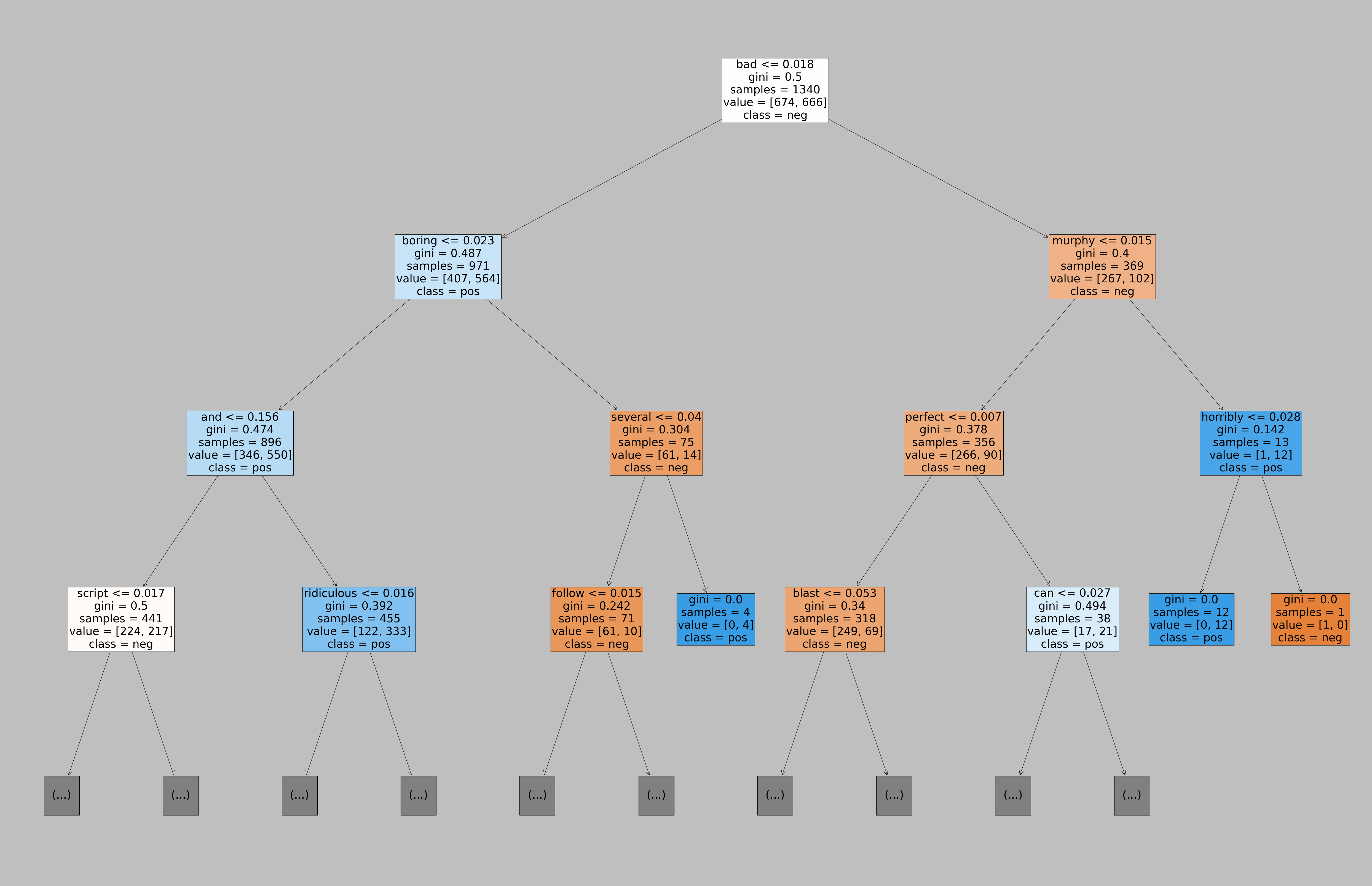
For tree-based classifiers, visualization is better.
import sklearn
from sklearn.tree import plot_tree
text_representation = sklearn.tree.export_text(model_dec, feature_names = tfidf_vec.get_feature_names_out().tolist())
print(text_representation)
|--- bad <= 0.02
|   |--- boring <= 0.02
|   |   |--- and <= 0.16
|   |   |   |--- script <= 0.02
|   |   |   |   |--- hilarious <= 0.01
|   |   |   |   |   |--- any <= 0.02
|   |   |   |   |   |   |--- if <= 0.02
|   |   |   |   |   |   |   |--- awful <= 0.02
|   |   |   |   |   |   |   |   |--- capsule <= 0.02
|   |   |   |   |   |   |   |   |   |--- reason <= 0.05
|   |   |   |   |   |   |   |   |   |   |--- class: pos
|   |   |   |   |   |   |   |   |   |--- reason >  0.05
|   |   |   |   |   |   |   |   |   |   |--- class: neg
|   |   |   |   |   |   |   |   |--- capsule >  0.02
|   |   |   |   |   |   |   |   |   |--- class: neg
|   |   |   |   |   |   |   |--- awful >  0.02
|   |   |   |   |   |   |   |   |--- class: neg
|   |   |   |   |   |   |--- if >  0.02
|   |   |   |   |   |   |   |--- into <= 0.02
|   |   |   |   |   |   |   |   |--- so <= 0.02
|   |   |   |   |   |   |   |   |   |--- becomes <= 0.01
|   |   |   |   |   |   |   |   |   |   |--- class: neg
|   |   |   |   |   |   |   |   |   |--- becomes >  0.01
|   |   |   |   |   |   |   |   |   |   |--- class: pos
|   |   |   |   |   |   |   |   |--- so >  0.02
|   |   |   |   |   |   |   |   |   |--- more <= 0.04
|   |   |   |   |   |   |   |   |   |   |--- class: pos
|   |   |   |   |   |   |   |   |   |--- more >  0.04
|   |   |   |   |   |   |   |   |   |   |--- class: neg
|   |   |   |   |   |   |   |--- into >  0.02
|   |   |   |   |   |   |   |   |--- class: neg
|   |   |   |   |   |--- any >  0.02
|   |   |   |   |   |   |--- performances <= 0.02
|   |   |   |   |   |   |   |--- life <= 0.03
|   |   |   |   |   |   |   |   |--- view <= 0.01
|   |   |   |   |   |   |   |   |   |--- itself <= 0.04
|   |   |   |   |   |   |   |   |   |   |--- class: neg
|   |   |   |   |   |   |   |   |   |--- itself >  0.04
|   |   |   |   |   |   |   |   |   |   |--- class: pos
|   |   |   |   |   |   |   |   |--- view >  0.01
|   |   |   |   |   |   |   |   |   |--- class: pos
|   |   |   |   |   |   |   |--- life >  0.03
|   |   |   |   |   |   |   |   |--- films <= 0.03
|   |   |   |   |   |   |   |   |   |--- class: pos
|   |   |   |   |   |   |   |   |--- films >  0.03
|   |   |   |   |   |   |   |   |   |--- class: neg
|   |   |   |   |   |   |--- performances >  0.02
|   |   |   |   |   |   |   |--- her <= 0.08
|   |   |   |   |   |   |   |   |--- class: pos
|   |   |   |   |   |   |   |--- her >  0.08
|   |   |   |   |   |   |   |   |--- class: neg
|   |   |   |   |--- hilarious >  0.01
|   |   |   |   |   |--- year <= 0.04
|   |   |   |   |   |   |--- ridiculous <= 0.05
|   |   |   |   |   |   |   |--- class: pos
|   |   |   |   |   |   |--- ridiculous >  0.05
|   |   |   |   |   |   |   |--- class: neg
|   |   |   |   |   |--- year >  0.04
|   |   |   |   |   |   |--- class: neg
|   |   |   |--- script >  0.02
|   |   |   |   |--- gain <= 0.02
|   |   |   |   |   |--- than <= 0.04
|   |   |   |   |   |   |--- feature <= 0.03
|   |   |   |   |   |   |   |--- love <= 0.07
|   |   |   |   |   |   |   |   |--- moments <= 0.07
|   |   |   |   |   |   |   |   |   |--- class: neg
|   |   |   |   |   |   |   |   |--- moments >  0.07
|   |   |   |   |   |   |   |   |   |--- class: pos
|   |   |   |   |   |   |   |--- love >  0.07
|   |   |   |   |   |   |   |   |--- class: pos
|   |   |   |   |   |   |--- feature >  0.03
|   |   |   |   |   |   |   |--- succeed <= 0.03
|   |   |   |   |   |   |   |   |--- class: pos
|   |   |   |   |   |   |   |--- succeed >  0.03
|   |   |   |   |   |   |   |   |--- class: neg
|   |   |   |   |   |--- than >  0.04
|   |   |   |   |   |   |--- with <= 0.05
|   |   |   |   |   |   |   |--- plot <= 0.01
|   |   |   |   |   |   |   |   |--- class: neg
|   |   |   |   |   |   |   |--- plot >  0.01
|   |   |   |   |   |   |   |   |--- class: pos
|   |   |   |   |   |   |--- with >  0.05
|   |   |   |   |   |   |   |--- class: pos
|   |   |   |   |--- gain >  0.02
|   |   |   |   |   |--- class: pos
|   |   |--- and >  0.16
|   |   |   |--- ridiculous <= 0.02
|   |   |   |   |--- minute <= 0.02
|   |   |   |   |   |--- then <= 0.04
|   |   |   |   |   |   |--- b <= 0.04
|   |   |   |   |   |   |   |--- forgot <= 0.03
|   |   |   |   |   |   |   |   |--- arms <= 0.04
|   |   |   |   |   |   |   |   |   |--- better <= 0.05
|   |   |   |   |   |   |   |   |   |   |--- class: pos
|   |   |   |   |   |   |   |   |   |--- better >  0.05
|   |   |   |   |   |   |   |   |   |   |--- class: neg
|   |   |   |   |   |   |   |   |--- arms >  0.04
|   |   |   |   |   |   |   |   |   |--- class: neg
|   |   |   |   |   |   |   |--- forgot >  0.03
|   |   |   |   |   |   |   |   |--- class: neg
|   |   |   |   |   |   |--- b >  0.04
|   |   |   |   |   |   |   |--- actor <= 0.02
|   |   |   |   |   |   |   |   |--- class: neg
|   |   |   |   |   |   |   |--- actor >  0.02
|   |   |   |   |   |   |   |   |--- class: pos
|   |   |   |   |   |--- then >  0.04
|   |   |   |   |   |   |--- quite <= 0.02
|   |   |   |   |   |   |   |--- habit <= 0.04
|   |   |   |   |   |   |   |   |--- class: neg
|   |   |   |   |   |   |   |--- habit >  0.04
|   |   |   |   |   |   |   |   |--- class: pos
|   |   |   |   |   |   |--- quite >  0.02
|   |   |   |   |   |   |   |--- class: pos
|   |   |   |   |--- minute >  0.02
|   |   |   |   |   |--- black <= 0.02
|   |   |   |   |   |   |--- class: neg
|   |   |   |   |   |--- black >  0.02
|   |   |   |   |   |   |--- apparent <= 0.03
|   |   |   |   |   |   |   |--- class: pos
|   |   |   |   |   |   |--- apparent >  0.03
|   |   |   |   |   |   |   |--- class: neg
|   |   |   |--- ridiculous >  0.02
|   |   |   |   |--- seen <= 0.02
|   |   |   |   |   |--- class: neg
|   |   |   |   |--- seen >  0.02
|   |   |   |   |   |--- strength <= 0.03
|   |   |   |   |   |   |--- class: pos
|   |   |   |   |   |--- strength >  0.03
|   |   |   |   |   |   |--- class: neg
|   |--- boring >  0.02
|   |   |--- several <= 0.04
|   |   |   |--- follow <= 0.02
|   |   |   |   |--- escape <= 0.04
|   |   |   |   |   |--- words <= 0.04
|   |   |   |   |   |   |--- territory <= 0.02
|   |   |   |   |   |   |   |--- smooth <= 0.04
|   |   |   |   |   |   |   |   |--- class: neg
|   |   |   |   |   |   |   |--- smooth >  0.04
|   |   |   |   |   |   |   |   |--- class: pos
|   |   |   |   |   |   |--- territory >  0.02
|   |   |   |   |   |   |   |--- class: pos
|   |   |   |   |   |--- words >  0.04
|   |   |   |   |   |   |--- class: pos
|   |   |   |   |--- escape >  0.04
|   |   |   |   |   |--- class: pos
|   |   |   |--- follow >  0.02
|   |   |   |   |--- class: pos
|   |   |--- several >  0.04
|   |   |   |--- class: pos
|--- bad >  0.02
|   |--- murphy <= 0.02
|   |   |--- perfect <= 0.01
|   |   |   |--- blast <= 0.05
|   |   |   |   |--- edge <= 0.03
|   |   |   |   |   |--- stolen <= 0.03
|   |   |   |   |   |   |--- wonderfully <= 0.02
|   |   |   |   |   |   |   |--- plane <= 0.05
|   |   |   |   |   |   |   |   |--- admit <= 0.04
|   |   |   |   |   |   |   |   |   |--- fest <= 0.02
|   |   |   |   |   |   |   |   |   |   |--- class: neg
|   |   |   |   |   |   |   |   |   |--- fest >  0.02
|   |   |   |   |   |   |   |   |   |   |--- class: pos
|   |   |   |   |   |   |   |   |--- admit >  0.04
|   |   |   |   |   |   |   |   |   |--- class: pos
|   |   |   |   |   |   |   |--- plane >  0.05
|   |   |   |   |   |   |   |   |--- class: pos
|   |   |   |   |   |   |--- wonderfully >  0.02
|   |   |   |   |   |   |   |--- class: pos
|   |   |   |   |   |--- stolen >  0.03
|   |   |   |   |   |   |--- ago <= 0.03
|   |   |   |   |   |   |   |--- class: pos
|   |   |   |   |   |   |--- ago >  0.03
|   |   |   |   |   |   |   |--- class: neg
|   |   |   |   |--- edge >  0.03
|   |   |   |   |   |--- montage <= 0.03
|   |   |   |   |   |   |--- class: pos
|   |   |   |   |   |--- montage >  0.03
|   |   |   |   |   |   |--- class: neg
|   |   |   |--- blast >  0.05
|   |   |   |   |--- class: pos
|   |   |--- perfect >  0.01
|   |   |   |--- can <= 0.03
|   |   |   |   |--- just <= 0.02
|   |   |   |   |   |--- michael <= 0.01
|   |   |   |   |   |   |--- class: pos
|   |   |   |   |   |--- michael >  0.01
|   |   |   |   |   |   |--- class: neg
|   |   |   |   |--- just >  0.02
|   |   |   |   |   |--- class: neg
|   |   |   |--- can >  0.03
|   |   |   |   |--- painfully <= 0.02
|   |   |   |   |   |--- class: pos
|   |   |   |   |--- painfully >  0.02
|   |   |   |   |   |--- class: neg
|   |--- murphy >  0.02
|   |   |--- horribly <= 0.03
|   |   |   |--- class: pos
|   |   |--- horribly >  0.03
|   |   |   |--- class: neg
plt.style.use('classic')
from matplotlib import pyplot as plt

fig = plt.figure(figsize=(80,50))
_ = sklearn.tree.plot_tree(model_dec, max_depth=3,
                   feature_names=tfidf_vec.get_feature_names_out().tolist(),  ## parameter requires list
                   class_names=model_dec.classes_.tolist(), ## parameter requires list
                   filled=True, fontsize=36)

#fig.savefig("decistion_tree.png")
Saving Model#
#  import pickle

# with open('../ml-sent-svm.pkl', 'wb') as f:
#     pickle.dump(clf, f)
# with open('../ml-sent-svm.pkl' 'rb') as f:
#     loaded_svm = pickle.load(f)
Dictionary-based Sentiment Classifier (Self-Study)#
Without machine learning, we can still build a sentiment classifier using a dictionary-based approach.
Words can be manually annotated with sentiment polarity scores.
Based on the sentiment dictionary, we can then compute the sentiment scores for a text.
TextBlob Lexicon#
from textblob import TextBlob
doc_sent = TextBlob(X_train[0])
print(doc_sent.sentiment)
print(doc_sent.sentiment.polarity)
Sentiment(polarity=0.15877050157184083, subjectivity=0.5661635487528345)
0.15877050157184083
doc_sents = [TextBlob(doc).sentiment.polarity for doc in X_train]
y_train[:10]
['neg', 'pos', 'pos', 'neg', 'pos', 'pos', 'neg', 'pos', 'neg', 'pos']
doc_sents_prediction = ['pos' if score >= 0.1 else 'neg' for score in doc_sents]
doc_sents_prediction[:10]
['pos', 'neg', 'pos', 'pos', 'pos', 'pos', 'neg', 'pos', 'neg', 'neg']
from sklearn.metrics import accuracy_score, f1_score, confusion_matrix, ConfusionMatrixDisplay
print(accuracy_score(y_train, doc_sents_prediction))
print(f1_score(y_train, doc_sents_prediction, average=None, labels=['neg','pos']))
0.7425373134328358
[0.74872542 0.73603673]
ConfusionMatrixDisplay(confusion_matrix(y_train, doc_sents_prediction, normalize="all"), display_labels=['neg','pos']).plot()
<sklearn.metrics._plot.confusion_matrix.ConfusionMatrixDisplay at 0x2d062ba60>
AFINN Lexicon#
from afinn import Afinn
afn = Afinn(emoticons=True)

afn.score("This movie, not good. worth it :( But can give it a try!! worth it")
0.0
doc_sents_afn = [afn.score(d) for d in X_train]
doc_sents_afn_prediction = ['pos' if score >= 1.0 else 'neg' for score in doc_sents_afn]
print(accuracy_score(y_train, doc_sents_afn_prediction))
print(f1_score(y_train, doc_sents_afn_prediction, average=None, labels=['neg','pos']))
0.6686567164179105
[0.61458333 0.70942408]
ConfusionMatrixDisplay(confusion_matrix(y_train, doc_sents_afn_prediction, normalize="all"),display_labels=['neg','pos']).plot()
<sklearn.metrics._plot.confusion_matrix.ConfusionMatrixDisplay at 0x2c9ab9160>
Disadvantage of Dictionary-based Approach
Constructing the sentiment dictionary is time-consuming.
The sentiment dictionary can be topic-dependent.
Package Requirement#
afinn==0.1
lime==0.2.0.1
matplotlib==3.7.2
nltk==3.8.1
numpy==1.24.3
pandas==2.0.3
scikit-learn==1.3.0
seaborn==0.12.2
textblob==0.17.1
References#
Geron (2019), Ch 2 and 3
Sarkar (2019), Ch 9
See a blog post, LIME of words: Interpreting RNN Predictions.
See a blog post, LIME of words: how to interpret your machine learning model predictions