
Machine Learning: A Simple Example#
Contents
A Quick Example: Name Gender Prediction#
Let’s assume that we have collected a list of personal names and we have their corresponding gender labels, i.e., whether the name is a male or female one.
The goal of this example is to create a classifier that would automatically classify a given name into either male or female.
Prepare Data#
We use the data provided in NLTK. Please download the corpus data if necessary.
We load the corpus,
nltk.corpus.namesand randomize it before we proceed.
import numpy as np
import nltk
from nltk.corpus import names
from nltk.classify import apply_features
import random
## Colab Only
nltk.download("names")
[nltk_data] Downloading package names to /root/nltk_data...
[nltk_data]   Unzipping corpora/names.zip.
True
labeled_names = ([(name, 'male') for name in names.words('male.txt')] +
                 [(name, 'female') for name in names.words('female.txt')])
random.shuffle(labeled_names)
Feature Engineering#
Now our base unit for classification is a name.
In feature engineering, our goal is to transform the texts (i.e., names) into vectorized representations.
To start with, let’s represent each text (name) by using its last character as the features.
def text_vectorizer(word):
    return {'last_letter': word[-1]}


text_vectorizer('Shrek')
{'last_letter': 'k'}
Train-Test Split#
We then apply the feature engineering method to every text in the data and split the data into training and testing sets.
featuresets = [(text_vectorizer(n), gender) for (n, gender) in labeled_names]
train_set, test_set = featuresets[500:], featuresets[:500]
Now all the training/testing tokens are included in a list.
Each training token (i.e., base unit) is encoded as a tuple of
(feature dictionary, string), where we have its features represented as a dictionary, and its label as a string.
train_set[:5]
[({'last_letter': 'd'}, 'male'),
 ({'last_letter': 'g'}, 'male'),
 ({'last_letter': 'i'}, 'male'),
 ({'last_letter': 'a'}, 'female'),
 ({'last_letter': 'a'}, 'female')]
Please note that in
NLTK, we can use theapply_featuresto create training and testing datasets.When you have a very large feature set, this can be more effective in terms of memory management.
This is our earlier method of creating training and testing sets:
featuresets = [(text_vectorizer(n), gender) for (n, gender) in labeled_names]
train_set, test_set = featuresets[500:], featuresets[:500]
# train_set = apply_features(text_vectorizer, labeled_names[500:])
# test_set = apply_features(text_vectorizer, labeled_names[:500])
Train the Model#
A good start is to try the simple Naive Bayes Classifier.
classifier = nltk.NaiveBayesClassifier.train(train_set)
Evaluate the Model#
After we train the model, we need to evaluate its performance on the testing dataset.
Model evaluation usually involves comparing the predictions provided by the model with the correct answers/labels.
The evaluation results are often summarized in a confusion matrix.
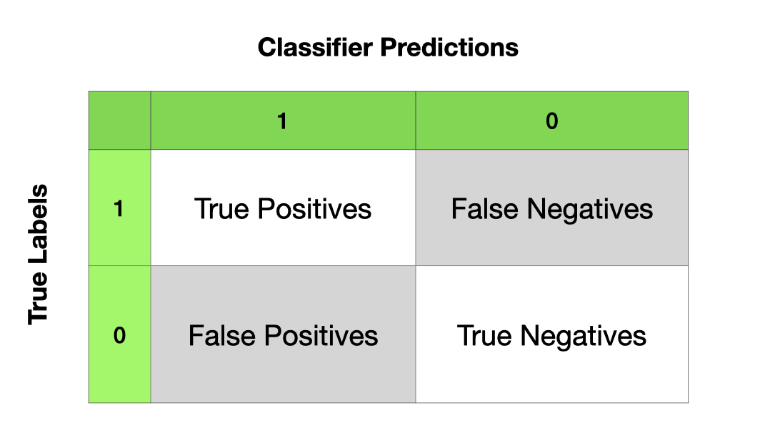
Confusion Matrix:
True positives are relevant items that we correctly identified as relevant.
True negatives are irrelevant items that we correctly identified as irrelevant.
False positives (or Type I errors) are irrelevant items that we incorrectly identified as relevant.
False negatives (or Type II errors) are relevant items that we incorrectly identified as irrelevant.
Given these four numbers, we can define the following model evaluation metrics:
Accuracy: How many items were correctly classified, i.e., \(\frac{TP + TN}{N}\)
Precision: How many of the items identified by the classifier as relevant are indeed relevant, i.e., \(\frac{TP}{TP+FP}\).
Recall: How many of the true relevant items were successfully identified by the classifier, i.e., \(\frac{TP}{TP+FN}\).
F-Measure (or F-Score): the harmonic mean of the precision and recall,i.e.:
\[ F= \frac{(2 × Precision × Recall)}{(Precision + Recall)} \]
Note
When dealing with imbalanced class distributions, we need to take into account the baseline performance in our model evaluation. For example. if the distribution of Class 0 and Class 1 is 9:1, then a naive classifier might as well classify all cases as Class 0, yielding a high-precision performance (i.e., Precision = 90%).
Given this baseline, to better evaluate the classifier on imbalanced dataset, probably the classifier’s recall rates are more important.
Note
Precision, Recall, and F-measure
In machine learning, precision and recall are two important metrics used to evaluate the performance of a classifier. Precision measures the proportion of correctly predicted positive instances among all instances predicted as positive, while recall measures the proportion of correctly predicted positive instances among all actual positive instances. Sometimes, it’s challenging to optimize both precision and recall simultaneously during model training because increasing one may lead to a decrease in the other. For example, making the classifier more conservative can improve precision but lower recall, and vice versa. This trade-off between precision and recall highlights the importance of using a metric that considers both aspects simultaneously, such as the F measure. The F measure combines precision and recall into a single score, providing a balanced assessment of a classifier’s performance without favoring one metric over the other. Therefore, in scenarios where precision and recall cannot be optimized simultaneously, the F measure becomes crucial for evaluating the classifier’s effectiveness.
print('Accuracy: {:4.2f}'.format(nltk.classify.accuracy(classifier, test_set)))
Accuracy: 0.74
## Compute the Confusion Matrix
t_f = [feature for (feature, label) in test_set]  # features of test set
t_l = [label for (feature, label) in test_set]  # labels of test set
t_l_pr = [classifier.classify(f) for f in t_f]  # predicted labels of test set
cm = nltk.ConfusionMatrix(t_l, t_l_pr)
cm = nltk.ConfusionMatrix(t_l, t_l_pr)
print(cm.pretty_format(sort_by_count=True, show_percents=False, truncate=9))
print(cm.pretty_format(sort_by_count=True, show_percents=True, truncate=9))
       |   f     |
       |   e     |
       |   m   m |
       |   a   a |
       |   l   l |
       |   e   e |
-------+---------+
female |<246> 60 |
  male |  71<123>|
-------+---------+
(row = reference; col = test)

       |      f        |
       |      e        |
       |      m      m |
       |      a      a |
       |      l      l |
       |      e      e |
-------+---------------+
female | <49.2%> 12.0% |
  male |  14.2% <24.6%>|
-------+---------------+
(row = reference; col = test)
## wrap as a function
def createCM(classifier, test_set):
    t_f = [feature for (feature, label) in test_set]
    t_l = [label for (feature, label) in test_set]
    t_l_pr = [classifier.classify(f) for f in t_f]
    cm = nltk.ConfusionMatrix(t_l, t_l_pr)
    print(cm.pretty_format(sort_by_count=True, show_percents=True, truncate=9))
createCM(classifier, test_set)
       |      f        |
       |      e        |
       |      m      m |
       |      a      a |
       |      l      l |
       |      e      e |
-------+---------------+
female | <49.2%> 12.0% |
  male |  14.2% <24.6%>|
-------+---------------+
(row = reference; col = test)
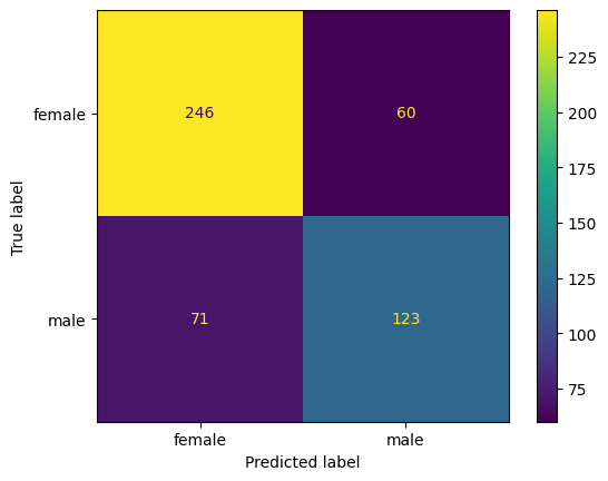
We can also get confusion matrix statistics from
sklearn:confusion_matrixConfusionMatrixDisplayclassification_report
from sklearn.metrics import classification_report, confusion_matrix, ConfusionMatrixDisplay
import matplotlib.pyplot as plt

## label names
target_names = ['female', 'male']
## confusion matrix
cm = confusion_matrix(y_true = t_l, y_pred = t_l_pr, labels = target_names)
print(cm)
## plotting
disp = ConfusionMatrixDisplay(confusion_matrix= cm,
                              display_labels= target_names)

disp.plot()
plt.show()
[[246  60]
 [ 71 123]]
## confusion matrix report
print(classification_report(y_true = t_l, y_pred = t_l_pr, target_names= ['female','male']))
              precision    recall  f1-score   support

      female       0.78      0.80      0.79       306
        male       0.67      0.63      0.65       194

    accuracy                           0.74       500
   macro avg       0.72      0.72      0.72       500
weighted avg       0.74      0.74      0.74       500
## Accuracy
print((272+124)/500)

## macro F measures
print((0.84 + 0.70)/2)

## weighted F measures
print(0.84*(315/(315+185)) + 0.70 * (185/(315+185)))
0.792
0.77
0.7882
Note
The macro-averaged F1 score (or macro F1 score) is computed using the arithmetic mean (aka unweighted mean) of all the per-class F1 scores. This method treats all classes equally regardless of their class distributions.
The weighted-averaged F1 score is calculated by taking the mean of all per-class F1 scores while considering each class’s distribution in the dataset. The “weight” essentially refers to the proportion of each class’s token numbers relative to the sum of the entire dataset.
Which metrics should be more crucial to your evaluation?
If you’re dealing with an imbalanced dataset where all classes are equally important, go for the macro-averaged F1 score.
If your dataset is imbalanced, but you want to give more importance to classes with more examples, go for the weighted-averaged F1 score.
If you have a balanced dataset and want a straightforward metric for overall performance, you can use accuracy, which is sometimes referred to as micro F1 score.
Model Prediction#
After we obtain a classifier, we can use it for (new) case predictions.
print(classifier.classify(text_vectorizer('Alvino')))
print(classifier.classify(text_vectorizer('Trinity')))
male
female
Post-hoc Analysis (Interpreting the model)#
One of the most important steps after model training is to examine which features contribute the most to the classifier prediction of the class.
classifier.show_most_informative_features(10)
Most Informative Features
             last_letter = 'a'            female : male   =     34.3 : 1.0
             last_letter = 'k'              male : female =     31.4 : 1.0
             last_letter = 'v'              male : female =     18.8 : 1.0
             last_letter = 'f'              male : female =     16.7 : 1.0
             last_letter = 'p'              male : female =     12.6 : 1.0
             last_letter = 'd'              male : female =     10.6 : 1.0
             last_letter = 'm'              male : female =      8.8 : 1.0
             last_letter = 'o'              male : female =      8.0 : 1.0
             last_letter = 'r'              male : female =      7.1 : 1.0
             last_letter = 'g'              male : female =      5.5 : 1.0
How can we improve the model/classifier?#
In the following, we will talk about methods that we may consider to further improve the model training.
Feature Engineering
Error Analysis
Cross Validation
Try Different Machine-Learning Algorithms
(Ensemble Methods)
More Sophisticated Feature Engineering#
We can extract more useful features from the names.
Use the following features for vectorized representations of names:
The first/last letter
Frequencies of all 26 alphabets in the names
## refine out text vectorizer
def text_vectorizer2(name):
    features = {}
    features["first_letter"] = name[0].lower()
    features["last_letter"] = name[-1].lower()
    for letter in 'abcdefghijklmnopqrstuvwxyz':
        features["count({})".format(letter)] = name.lower().count(letter)
        features["has({})".format(letter)] = (letter in name.lower())
    return features
text_vectorizer2('Alvin')
{'first_letter': 'a',
 'last_letter': 'n',
 'count(a)': 1,
 'has(a)': True,
 'count(b)': 0,
 'has(b)': False,
 'count(c)': 0,
 'has(c)': False,
 'count(d)': 0,
 'has(d)': False,
 'count(e)': 0,
 'has(e)': False,
 'count(f)': 0,
 'has(f)': False,
 'count(g)': 0,
 'has(g)': False,
 'count(h)': 0,
 'has(h)': False,
 'count(i)': 1,
 'has(i)': True,
 'count(j)': 0,
 'has(j)': False,
 'count(k)': 0,
 'has(k)': False,
 'count(l)': 1,
 'has(l)': True,
 'count(m)': 0,
 'has(m)': False,
 'count(n)': 1,
 'has(n)': True,
 'count(o)': 0,
 'has(o)': False,
 'count(p)': 0,
 'has(p)': False,
 'count(q)': 0,
 'has(q)': False,
 'count(r)': 0,
 'has(r)': False,
 'count(s)': 0,
 'has(s)': False,
 'count(t)': 0,
 'has(t)': False,
 'count(u)': 0,
 'has(u)': False,
 'count(v)': 1,
 'has(v)': True,
 'count(w)': 0,
 'has(w)': False,
 'count(x)': 0,
 'has(x)': False,
 'count(y)': 0,
 'has(y)': False,
 'count(z)': 0,
 'has(z)': False}
text_vectorizer2('John')
{'first_letter': 'j',
 'last_letter': 'n',
 'count(a)': 0,
 'has(a)': False,
 'count(b)': 0,
 'has(b)': False,
 'count(c)': 0,
 'has(c)': False,
 'count(d)': 0,
 'has(d)': False,
 'count(e)': 0,
 'has(e)': False,
 'count(f)': 0,
 'has(f)': False,
 'count(g)': 0,
 'has(g)': False,
 'count(h)': 1,
 'has(h)': True,
 'count(i)': 0,
 'has(i)': False,
 'count(j)': 1,
 'has(j)': True,
 'count(k)': 0,
 'has(k)': False,
 'count(l)': 0,
 'has(l)': False,
 'count(m)': 0,
 'has(m)': False,
 'count(n)': 1,
 'has(n)': True,
 'count(o)': 1,
 'has(o)': True,
 'count(p)': 0,
 'has(p)': False,
 'count(q)': 0,
 'has(q)': False,
 'count(r)': 0,
 'has(r)': False,
 'count(s)': 0,
 'has(s)': False,
 'count(t)': 0,
 'has(t)': False,
 'count(u)': 0,
 'has(u)': False,
 'count(v)': 0,
 'has(v)': False,
 'count(w)': 0,
 'has(w)': False,
 'count(x)': 0,
 'has(x)': False,
 'count(y)': 0,
 'has(y)': False,
 'count(z)': 0,
 'has(z)': False}
## more sophisticated feature engineering
train_set = apply_features(text_vectorizer2, labeled_names[500:])
test_set = apply_features(text_vectorizer2, labeled_names[:500])
## train the model
classifier = nltk.NaiveBayesClassifier.train(train_set)
## evaluate the model
print(nltk.classify.accuracy(classifier, test_set))
0.76
## Post-hoc analysis
classifier.show_most_informative_features(n=20)
Most Informative Features
             last_letter = 'a'            female : male   =     34.3 : 1.0
             last_letter = 'k'              male : female =     31.4 : 1.0
             last_letter = 'v'              male : female =     18.8 : 1.0
             last_letter = 'f'              male : female =     16.7 : 1.0
             last_letter = 'p'              male : female =     12.6 : 1.0
             last_letter = 'd'              male : female =     10.6 : 1.0
                count(v) = 2              female : male   =      9.2 : 1.0
             last_letter = 'm'              male : female =      8.8 : 1.0
             last_letter = 'o'              male : female =      8.0 : 1.0
             last_letter = 'r'              male : female =      7.1 : 1.0
             last_letter = 'g'              male : female =      5.5 : 1.0
             last_letter = 'w'              male : female =      5.1 : 1.0
            first_letter = 'w'              male : female =      4.6 : 1.0
             last_letter = 's'              male : female =      4.5 : 1.0
                count(a) = 3              female : male   =      4.4 : 1.0
                count(w) = 1                male : female =      4.3 : 1.0
                  has(w) = True             male : female =      4.3 : 1.0
             last_letter = 'j'              male : female =      4.0 : 1.0
                count(o) = 2                male : female =      3.7 : 1.0
             last_letter = 'i'            female : male   =      3.7 : 1.0
Train-Development-Test Data Splits for Error Analysis#
Normally we have training-testing splits of data
Sometimes we can use development (dev) set for error analysis and feature engineering.
This dev set should be independent of training and testing sets.
Now let’s train the model on the training set and first check the classifier’s performance on the dev set.
We then identify the errors the classifier made in the dev set.
We perform error analysis for potential model improvement.
We only test our final model on the testing set. (Note: Testing set can only be used once.)
## train-dev-test split
train_names = labeled_names[1500:]
devtest_names = labeled_names[500:1500]
test_names = labeled_names[:500]

## Feature engineering
train_set = [(text_vectorizer2(n), gender) for (n, gender) in train_names]
devtest_set = [(text_vectorizer2(n), gender) for (n, gender) in devtest_names]
test_set = [(text_vectorizer2(n), gender) for (n, gender) in test_names]

## Train the model
classifier = nltk.NaiveBayesClassifier.train(train_set)

## Evaluate the model on dev set
print(nltk.classify.accuracy(classifier, devtest_set))
0.78
## identify error cases

errors = []
for (name, tag) in devtest_names:
    guess = classifier.classify(text_vectorizer2(name))
    if guess != tag:
        errors.append((tag, guess, name))
## save error cases for post-hoc analysis
import csv

with open('error-analysis.csv', 'w') as f:

    # using csv.writer method from CSV package
    write = csv.writer(f)
    write.writerow(['tag', 'guess', 'name'])
    write.writerows(errors)
Ideally, we can inspect the errors in a spreadsheet and come up with better rules (features) that could help improve the classifier.
import pandas as pd
## check first and last N rows
pd.read_csv('error-analysis.csv').iloc[[*range(10), *range(-10, 0)],]
| tag | guess | name | |
|---|---|---|---|
| 0 | male | female | Barri |
| 1 | female | male | Dorolice |
| 2 | female | male | Gwennie |
| 3 | female | male | Honey |
| 4 | female | male | Rosaleen |
| 5 | male | female | Max |
| 6 | male | female | Sinclare |
| 7 | male | female | Costa |
| 8 | male | female | Archie |
| 9 | female | male | Margaux |
| 210 | female | male | Fortune |
| 211 | male | female | Gayle |
| 212 | male | female | Parke |
| 213 | male | female | Matthias |
| 214 | male | female | Lazar |
| 215 | male | female | Nate |
| 216 | male | female | Avi |
| 217 | female | male | Hesther |
| 218 | female | male | Tori |
| 219 | female | male | Norry |
Cross Validation#
We can also check our average model performance using the cross-validation method on the training dataset before the real testing of the model.
This method is often useful if you need to fine-tune the hyperparameters during the model training stage.
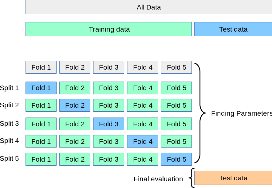 (Source: https://scikit-learn.org/stable/modules/cross_validation.html)
import sklearn.model_selection
kf = sklearn.model_selection.KFold(n_splits=10)
acc_kf = []  ## accuracy holder

## Cross-validation
for train_index, test_index in kf.split(train_set):
    #print("TRAIN:", train_index, "TEST:", test_index)
    classifier = nltk.NaiveBayesClassifier.train(
        train_set[train_index[0]:train_index[len(train_index) - 1]])
    cur_fold_acc = nltk.classify.util.accuracy(
        classifier, train_set[test_index[0]:test_index[len(test_index) - 1]])
    acc_kf.append(cur_fold_acc)
    print('accuracy:', np.round(cur_fold_acc, 2))
accuracy: 0.75
accuracy: 0.79
accuracy: 0.77
accuracy: 0.78
accuracy: 0.79
accuracy: 0.76
accuracy: 0.79
accuracy: 0.79
accuracy: 0.77
accuracy: 0.75
np.mean(acc_kf)
0.7752579137003371
Try Different Machine Learning Algorithms#
There are many ML algorithms for classification tasks.
Here we will demonstrate a few more classifiers implemented in NLTK, including:
Maximum Entropy Classifier (Logistic Regression)
Decision Tree Classifier
Also, in NLTK, we can use the classification methods provided in
sklearnas well, including:Naive Bayes
Logistic Regression
Support Vector Machine
When we try another ML algorithm, we do the following:
train the model
check model performance (accuracy and confusion matrix)
check the most informative features
obtain average performance using k-fold cross validation
Try Maxent Classifier#
Maxent is memory hungry, slower, and it requires
numpy.
%%time
from nltk.classify import MaxentClassifier

## Train Maxent model
classifier_maxent = MaxentClassifier.train(train_set,
                                           algorithm='iis',
                                           trace=0,
                                           max_iter=10000,
                                           min_lldelta=0.001)
CPU times: user 2min 17s, sys: 321 ms, total: 2min 17s
Wall time: 2min 30s
Note
The default algorithm for training is iis (Improved Iterative Scaling). Another alternative is gis (General Iterative Scaling), which is faster.
%%time
## Cross validation on training
for train_index, test_index in kf.split(train_set):
    #print("TRAIN:", train_index, "TEST:", test_index)
    classifier = MaxentClassifier.train(
        train_set[train_index[0]:train_index[len(train_index) - 1]],
        algorithm='gis',
        trace=0,
        max_iter=100,
        min_lldelta=0.01) ## set smaller value for `min_lldelta`
    print(
        'accuracy:',
        nltk.classify.util.accuracy(
            classifier,
            train_set[test_index[0]:test_index[len(test_index) - 1]]))
accuracy: 0.6645962732919255
accuracy: 0.6909937888198758
accuracy: 0.703416149068323
accuracy: 0.6987577639751553
accuracy: 0.7107309486780715
accuracy: 0.687402799377916
accuracy: 0.6982892690513219
accuracy: 0.7371695178849145
accuracy: 0.6827371695178849
accuracy: 0.7278382581648523
CPU times: user 2min 41s, sys: 386 ms, total: 2min 41s
Wall time: 2min 51s
## evaluate the model
createCM(classifier_maxent, test_set)
       |      f        |
       |      e        |
       |      m      m |
       |      a      a |
       |      l      l |
       |      e      e |
-------+---------------+
female | <52.2%>  9.0% |
  male |  12.6% <26.2%>|
-------+---------------+
(row = reference; col = test)
## posthoc analysis
classifier_maxent.show_most_informative_features(n=20)
  -3.144 last_letter=='a' and label is 'male'
  -2.263 last_letter=='k' and label is 'female'
  -2.106 last_letter=='v' and label is 'female'
  -2.056 count(v)==2 and label is 'male'
  -1.622 last_letter=='f' and label is 'female'
   1.420 count(j)==2 and label is 'female'
  -1.396 last_letter=='p' and label is 'female'
  -1.373 last_letter=='d' and label is 'female'
  -1.218 last_letter=='m' and label is 'female'
  -1.129 last_letter=='i' and label is 'male'
   1.040 last_letter=='c' and label is 'male'
  -1.037 count(y)==2 and label is 'male'
  -1.035 last_letter=='o' and label is 'female'
  -1.026 last_letter=='r' and label is 'female'
  -0.896 count(e)==4 and label is 'male'
  -0.888 last_letter=='b' and label is 'female'
  -0.870 last_letter=='g' and label is 'female'
   0.747 count(g)==3 and label is 'male'
  -0.696 last_letter=='s' and label is 'female'
  -0.681 count(e)==3 and label is 'male'
Try Decision Tree#
Parameters:
binary: whether the features are binaryentropy_cutoff: a value used during tree refinement processentropy = 1 -> high-level uncertainty
entropy = 0 -> perfect model prediction
depth_cutoff: to control the depth of the treesupport_cutoff: the minimum number of instances that are required to make a decision about a feature.
%%time
## Train decision tree model
from nltk.classify import DecisionTreeClassifier
classifier_dt = DecisionTreeClassifier.train(train_set,
                                             binary=True,
                                             entropy_cutoff=0.7,
                                             depth_cutoff=5,
                                             support_cutoff=5)
CPU times: user 18.9 s, sys: 44 ms, total: 18.9 s
Wall time: 19.1 s
%%time
## cross-validation on training
for train_index, test_index in kf.split(train_set):
    #print("TRAIN:", train_index, "TEST:", test_index)
    classifier = DecisionTreeClassifier.train(
        train_set[train_index[0]:train_index[len(train_index) - 1]],
        binary=True,
        entropy_cutoff=0.7,
        depth_cutoff=5,
        support_cutoff=5)
    print(
        'accuracy:',
        nltk.classify.util.accuracy(
            classifier,
            train_set[test_index[0]:test_index[len(test_index) - 1]]))
accuracy: 0.7080745341614907
accuracy: 0.7282608695652174
accuracy: 0.6987577639751553
accuracy: 0.6894409937888198
accuracy: 0.7480559875583204
accuracy: 0.7231726283048211
accuracy: 0.7620528771384136
accuracy: 0.7433903576982893
accuracy: 0.6982892690513219
accuracy: 0.7122861586314152
CPU times: user 2min 59s, sys: 408 ms, total: 3min
Wall time: 3min 2s
## evaluate the model on test data
createCM(classifier_dt, test_set)
       |      f        |
       |      e        |
       |      m      m |
       |      a      a |
       |      l      l |
       |      e      e |
-------+---------------+
female | <53.0%>  8.2% |
  male |  22.6% <16.2%>|
-------+---------------+
(row = reference; col = test)
## posthoc
print(classifier_dt.pretty_format(depth=5))
last_letter=d? ........................................ male
else: ................................................. male
  last_letter=r? ...................................... female
    count(n)=2? ....................................... female
      has(e)=False? ................................... male
      else: ........................................... female
        count(a)=1? ................................... male
        else: ......................................... female
    else: ............................................. male
  else: ............................................... male
    last_letter=s? .................................... female
      first_letter=p? ................................. male
        has(n)=False? ................................. female
        else: ......................................... male
      else: ........................................... female
        count(o)=2? ................................... female
        else: ......................................... male
    else: ............................................. male
      last_letter=o? .................................. male
      else: ........................................... female
        last_letter=n? ................................ male
        else: ......................................... female
Try sklearn Classifiers#
sklearnis a very useful module for machine learning. We will talk more about this module in our later lectures.This package provides a lot more ML algorithms for classification tasks.
Naive Bayes in sklearn#
from nltk.classify.scikitlearn import SklearnClassifier
from sklearn.naive_bayes import MultinomialNB


## Using sklearn naive bayes in nltk
sk_classifier = SklearnClassifier(MultinomialNB())
sk_classifier.train(train_set)
<SklearnClassifier(MultinomialNB())>
## evaluate model
nltk.classify.accuracy(sk_classifier, test_set)
0.746
Logistic Regression in sklearn#
from sklearn.linear_model import LogisticRegression

## using sklearn logistic regression in nltk
sk_classifier = SklearnClassifier(LogisticRegression(max_iter=500))
sk_classifier.train(train_set)

## evaluate the model
nltk.classify.accuracy(sk_classifier, test_set)
# createCM(sk_classifier, test_set)
0.78
Support Vector Machine in sklearn#
sklearnprovides several implementations for Support Vector Machines.Please see its documentation for more detail: Support Vector Machine
from sklearn.svm import SVC

## using sklearn SVM in nltk
sk_classifier = SklearnClassifier(SVC())
sk_classifier.train(train_set)

## evaluate the model
nltk.classify.accuracy(sk_classifier, test_set)
# createCM(sk_classifier, test_set)
0.81
from sklearn.svm import LinearSVC

## using sklearn linear SVM in nltk
sk_classifier = SklearnClassifier(LinearSVC(max_iter=2000, dual=True))
sk_classifier.train(train_set)

## evaluate model
nltk.classify.accuracy(sk_classifier, test_set)
0.774
from sklearn.svm import NuSVC

## using sklearn linear nuSVM in nltk
sk_classifier = SklearnClassifier(NuSVC())
sk_classifier.train(train_set)
## evaluate model
nltk.classify.accuracy(sk_classifier, test_set)
0.8
Remaining Issues#
Feature Engineering: Feature engineering is highlighted as a crucial aspect of the machine learning process. This involves selecting, extracting, and transforming features from the raw data to create meaningful representations that can improve the performance of the model.
Linguistically Motivated Features: There is a suggestion to include more linguistically motivated features during the feature engineering process. This implies that domain-specific knowledge and linguistic insights can be valuable in designing features that capture relevant information from the data.
Text Vectorization Quality: The quality of text vectorization is emphasized as it greatly influences the performance of the classifier. Text vectorization converts textual data into numerical representations that machine learning algorithms can work with. Ensuring accurate and informative vectorization is crucial for effective modeling.
Hyperparameter Tuning: Every machine learning algorithm requires setting hyperparameters, which can significantly impact the model’s performance. Tuning these hyperparameters to optimal values is essential for achieving the best possible performance from the model.
Systematic Hyperparameter Optimization: There is a need for a more systematic approach to finding the optimal combinations of hyperparameters for a given machine learning algorithm. This suggests the importance of methods such as grid search or randomized search to systematically explore the hyperparameter space and identify the best settings.
Importance of Sklearn: We will come back to these issues when discussing machine learning with
sklearn.
References#
NLTK Book, Chapter 6 Learning to Classify Texts
Géron (2019), Chapter 3 Classification