Chapter 4 Subsetting
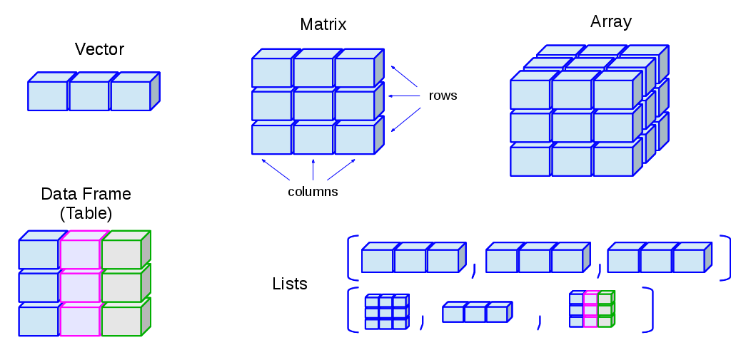
Subsetting is a crucial skill in data analysis. It involves selecting a specific subset of elements from a data structure such as a vector, matrix, data frame, or list. In Chapter 2, we provided a brief overview of data structures in R. In this section, we will delve deeper into each type of data structure and explore different techniques for subsetting them. By mastering subsetting, you will be able to efficiently extract the necessary information from your data for analysis and visualization.
In particular, we will look at three main topics:
- Subsetting: Subsetting refers to extracting specific elements from a larger data structure, such as a vector or a data frame, based on their position or label.
- Conditional Subsetting: Conditional subsetting involves extracting elements from a data structure based on some specific conditions or criteria.
- Sorting: Sorting involves ordering the elements of a data structure, such as a vector or a data frame, in a specific way based on their values.
4.1 Vector
Subsetting
As we have shown in Chapter 2 R Fundamentals, there are three types of primitive vectors in R:
- Character vectors
- Numeric vectors
- Boolean vectors
You can access a particular subset of a vector by using [ ] right after the object name. Within the [], you can make use of at least three types of indices:
- Subsetting with numeric indices
[1] "one"You can also retrieve several elements from a vector all at once, using a numeric vector as the indices, c(), in the []:
[1] "one" "four"[1] "one" "four"- Subsetting with Boolean indices
You can also use a Boolean vector as the index:
[1] "one" "three"[1] "one" "three"- Subsetting with negative numeric indices
If you use negative integers as indices within the square brackets, R will return a new vector with the elements at those indices removed. In other words, negative indexing allows you to exclude certain elements from the original vector. This is a useful technique for filtering out specific values or observations that you don’t need for a particular analysis or operation.
[1] "one" "three" "four" "five" However, please note that the original vector is still the same in length:
[1] "one" "two" "three" "four" "five" If you want to save the shortened/filtered vector, there are at least two alternatives:
- Assign the shortened vector to a new object name;
- Assign the shortened vector to the old object name.
[1] "one" "three" "four" "five" [1] "one" "two" "three" "four" "five" [1] "one" "three" "four" "five" For the two alternatives, which one would be better? Why?
The indices in R start with one, meaning that the first element of a vector or the first row/column of a matrix is indexed as one.
This is different from some other programming languages, such as Python, which use zero-based indexing, meaning that the first element of a vector or the first row/column of a matrix is indexed as zero.
It is important to be aware of this difference when working with data in R, especially if you are coming from a programming background that uses zero-based indexing. Using the wrong index can lead to unexpected results or errors in your code.
Conditional Subsetting
In R, we often need to extract specific elements from a data structure that meet certain conditions. We can achieve this by using conditional subsetting. One useful function for conditional subsetting is which().
which() returns the indices of the elements in a vector, matrix, or array that satisfy a certain condition. The condition can be specified using a logical expression, which returns a logical vector with TRUE for the elements that meet the condition and FALSE for those that do not.
For example, suppose we have a vector x that contains some values and we want to extract the indices of all the elements that are greater than 5. We can do this using the which() function in the following way:
Here, which(x > 5) returns the indices of the elements in x that are greater than 5, which are 2, 4, and 5. Therefore, indices contains the vector 2 4 5.
Once we have the indices of the elements that satisfy the condition, we can use them to subset the original data structure. For example, we can extract the elements of x that are greater than 5 as follows:
[1] 7 9 6[1] 7 9 6You may use different logical operators to check each element of the vector according to some criteria. R will decide whether elements of the vector satisfy the condition given in the logical expression and return a Boolean vector of the same length. Common logical operators include:
==: equal to&: and|: or>: greater than>=: greater than or equal to<: less than<=: less than or equal to!=: not equal
This can be very useful for vector conditional subsetting:
 [1] FALSE FALSE FALSE FALSE FALSE FALSE FALSE FALSE FALSE FALSE  TRUE  TRUE
[13] TRUE TRUE TRUE TRUE TRUE TRUE TRUE TRUE [1] 11 12 13 14 15 16 17 18 19 20 [1] 1 2 3 4 5 6 7 8 9 11 12 13 14 15 16 17 18 19 20We can also combine conditions using logical operators like & (and) and | (or). For example, if we want to check whether elements in a vector are greater than 18 or less than 2, we can use the | (or) operator to combine two conditions like this:
[1] 1 19 20Exercise 4.1 Use conditional subsetting to subset the strings in char.vec that meet the following conditions. Specifically, subset strings in char.vec that belong to either “one” or “three” using conditional subsetting. Your task is to find the right target.indices.
[1] "one" "three"Exercise 4.2 Use the sample() function to create a numeric vector, named num.vec, of length 10, containing 10 different integers randomly selected from the range 1 to 100. Then use conditional subsetting to subset only even numbers from the numeric vector. Your job is to find the right target.indices.
[1] 31 79 51 14 67 42 50 43 97 25[1] 14 42 50Sorting
Sorting elements from a data structure is a common task when working with data. The sort() and order() functions are useful for sorting elements in ascending or descending order based on their values.
- The
sort()function is used to sort elements in a data structure, such as a vector, matrix, or data frame. It arranges the elements in increasing or decreasing order, based on the values. - The
order()function is similar tosort(), but it returns the indices of the sorted elements, rather than the sorted elements themselves. This can be useful when we want to rearrange a data structure based on the order of its elements. The order() function also has optional arguments that can be used to customize the sorting process, such as specifying the sorting order and the way ties are handled.
[1] 1 3 5 7 9[1] 2 4 3 1 5[1] 1 3 5 7 9First, we used sort() to sort the elements of vec in ascending order. The resulting vector has the same elements as vec, but they are sorted from smallest to largest.
In the second example, we used order() to obtain the index positions that would sort vec in ascending order. We then used these index positions to subset the elements of vec in the desired order. This achieves the same result as using sort() directly.
Exercise 4.3 Create a vector, named m, which includes the lowercase letters from a to j in an alphabetical order.
- hint: You can do this by using the
letterspre-loaded R object to create a vector of all lowercase letters and then selecting the subset of letters fromatojusing the[ ]notation.
[1] "a" "b" "c" "d" "e" "f" "g" "h" "i" "j"Exercise 4.4 Create a vector n containing the same letters as m (from the previous exercise), but in a random order.
That is, create another vector, named n, which includes small letters from a to j (in a random order).
- hint: You can use the
sample()function for random sampling. Also, your results may vary because of the random ordering of the letters.
[1] "e" "h" "d" "i" "c" "a" "b" "g" "f" "j"Exercise 4.5 Determine whether the letters in n (i.e., the one with the random order) are in the same positions as they are in m (i.e., the one with the alphabetical order).
First, count how many letters are in the same position in n as they are in m; second, identify which letters are in the same position in both vectors.
- hint: check
table()
FALSE  TRUE
    9     1
[1] "j"4.2 Factor
In Chapter 2, we discussed several data structures in R, but one important structure that we did not cover is the factor. Factors are similar to vectors, but with an important difference: they have a limited number of possible values, called levels, which can be thought of as categories or groups. Factors are often used in statistical analysis as grouping variables, to separate observations into different sub-groups. In this section, we will explore the basics of factors and how to work with them in R.
We usually create a factor from a numeric or character vector. To create a factor, use factor():
[1] 1 0 0 1 1 0 1[1] 1 0 0 1 1 0 1
Levels: 0 1But please note that the numbers that you see in a factor do not represent numeric values. Instead, they are labels in the form of digits.
[1] "female" "male" "male" "female" "female" "male" "female"[1] female male male female female male female
Levels: female maleFor a factor, the most important information is its levels, i.e., the limited set of all possible values this factor can take. We can extract the levels as a vector of character strings using levels():
[1] "0" "1"[1] "female" "male" When do we need a factor? In data annotation, we often use arbitrary numbers as labels for certain categorical variables. For example, we may use arbitrary numbers from 1 to 4 to label learners’ varying proficiency levels: 1 = beginners, 2 = low-intermediate, 3 = upper-intermediate, 4 = advanced. When we load the data into R, R may first treat the data as a numeric vector:
[1] 1 2 4 4 2 3 3 1 1However, these numbers may be confusing:
- R may perform operations that make sense on numbers but may not make sense on categorical variables. For example, it doesn’t make sense to calculate the mean or the sum of categories such as “beginner”, “intermediate”, and “advanced”.
- They are not semantically transparent because numbers do not have meanings.
In this case, we can convert the numeric vector into a factor and re-label these numeric values as categorical labels that are more semantically transparent.
We can do this by setting more arguments in factor(), such as levels=..., labels=....
sbj_prof_fac <- factor(
  x = sbj_prof_num,
  levels = c(1:4),
  labels = c("beginner", "low-inter", "upper-inter", "advanced")
)
sbj_prof_fac
[1] beginner low-inter advanced advanced low-inter upper-inter
[7] upper-inter beginner beginner
Levels: beginner low-inter upper-inter advanced[1] 1 2 4 4 2 3 3 1 1Compare the the auto-print outputs of sbj_prof_fac and sbj_prof_num and examine their differences.
levels = ...: this argument specifies all possible values this factor can takelabels = ...: this argument provides own intuitive labels for each level
It should now therefore be clear that labels = ... is a good way for us to re-label any arbitrary annotations into meaningful labels. By using the levels and labels arguments, we can make the factors more intuitive and easier to understand, particularly if the original data uses arbitrary values or codes to represent categories.
In addition, we can determine whether the ranking of the levels is meaningful. If the order of the factor’s levels is meaningful, we can set the argument ordered = TRUE:
sbj_prof_fac_ordered <- factor(
  x = sbj_prof_num,
  levels = c(1:4),
  labels = c("beginner", "low-inter", "upper-inter", "advanced"),
  ordered = T
)
sbj_prof_fac_ordered
[1] beginner low-inter advanced advanced low-inter upper-inter
[7] upper-inter beginner beginner
Levels: beginner < low-inter < upper-inter < advancedNow from the R console we can see not only the levels of the factor but also the signs <, indicating their order. Using this ordered factor, we can perform relational comparison:
[1] beginner
Levels: beginner < low-inter < upper-inter < advanced[1] advanced
Levels: beginner < low-inter < upper-inter < advanced[1] TRUEBut we cannot do the comparison for unordered factors (characters neither):
[1] beginner
Levels: beginner low-inter upper-inter advanced[1] advanced
Levels: beginner low-inter upper-inter advancedWarning in Ops.factor(sbj_prof_fac[1], sbj_prof_fac[4]): '<' not meaningful for
factors[1] NAThe difference between vector and factor may look trivial for the moment but they are statistically very crucial. The choice of whether to instruct R to treat a vector as a factor, or even an ordered factor, will have important consequences in the implementation of many statistical methods, such as regression or other generalized linear modeling.
Rule of thumb: Always pay attention to what kind of object class you are dealing with:)
4.3 List
A List is like a vector, which is a one-dimensional data structure. However, the main difference is that a List can include a series of objects of different classes:
# A list consists of
# (i) numeric vector,
# (ii) character vector,
# (iii) Boolean vector
list.example <- list(
  "one" = c(1, 2, 3),
  "two" = c("Joe", "Mary", "John", "Angela"),
  "three" = c(TRUE, TRUE)
)

list.example
$one
[1] 1 2 3
$two
[1] "Joe" "Mary" "John" "Angela"
$three
[1] TRUE TRUEPlease note that not only the class of each object in the List does not have to be the same; the length of each list element may also vary.
You can subset a List in two ways:
[...]: This always returns aListback[[...]]: This returns the object of theListelement, which is NOT NECESSARILY aList
$one
[1] 1 2 3[1] 1 2 3[1] 1 2 3We can also subset a List by the names of its elements.
Before you try the following codes in the R console, could you first predict the outputs?
Exercise 4.6 Create a list that contains, in this order:
- a sequence of 20 evenly spaced numbers between -4 and 4; (hint: check
seq()) - a 3 x 3 matrix of the logical vector
c(F,T,T,T,F,T,T,F,F)filled column-wise; - a character vector with the two strings “don”, and “quixote”;
- a factor containing the observations
c("LOW","MID","LOW","MID","MID","HIGH").
[[1]]
 [1] -4.0000000 -3.5789474 -3.1578947 -2.7368421 -2.3157895 -1.8947368
 [7] -1.4736842 -1.0526316 -0.6315789 -0.2105263  0.2105263  0.6315789
[13]  1.0526316  1.4736842  1.8947368  2.3157895  2.7368421  3.1578947
[19]  3.5789474  4.0000000

[[2]]
      [,1]  [,2]  [,3]
[1,] FALSE  TRUE  TRUE
[2,]  TRUE FALSE FALSE
[3,]  TRUE  TRUE FALSE

[[3]]
[1] "don"     "quixote"

[[4]]
[1] LOW  MID  LOW  MID  MID  HIGH
Levels: HIGH LOW MID
Exercise 4.7 Based on Exercise 4.6, extract row elements 2 and 1 of columns 2 and 3, in that order, of the logical matrix.
      [,1]  [,2]
[1,] FALSE FALSE
[2,]  TRUE  TRUE
Exercise 4.8 Based on Exercise 4.6, obtain all values from the sequence between -4 and 4 that are greater than 1.
[1] 1.052632 1.473684 1.894737 2.315789 2.736842 3.157895 3.578947 4.000000Exercise 4.9 Make yourself familiar with the function which(). Based on Exercise 4.6, use which(), to determine which indices in the factor are assigned the “MID” level.
[1] 2 4 54.4 Data Frame
Subsetting
A data.frame is the most frequently used object that we will work with in data analysis. It is a typical two-dimensional spreadsheet-like table. Normally, the rows are the subjects or tokens we are analyzing; the columns are the variables or factors we are interested in.
We can also use [... , ... ] to subset a data frame. The indices in [... , ...] are Row-by-Column.
ex_df <- data.frame(
  WORD = c("the", "boy", "you","him"),
  POS = c("ART","N","PRO","PRO"),
  FREQ = c(1104,35, 104, 34)
)
ex_df
You can subset a particular row of the data frame:
You can subset a particular column of the data frame:
[1] "the" "boy" "you" "him"Please compare the following two ways of accessing a column from the data frame. Can you tell the differences in the returned results?
[1] 1104 35 104 34Conditional Subsetting
We can also make use of which() to perform conditional subsetting.
Can you subset rows whose FREQ < 50?
Can you subset rows whose POS are either PRO or N?
Sorting
We can also make use of order() to sort the data frame into a specific order based on the values of the columns.
Can you sort the data frame ex_df based on the values of the column WORD, arranging the rows in descending alphabetical order?”
Can you sort the data frame ex_df based on the values of the column FREQ in descending order.
Exercise 4.10 Create and store the following data frame as dframe in your R workspace.
personshould be a character vectorsexshould be a factor with levelsFandMfunnyshould be a factor with levelsLow,Mid, andHigh
Exercise 4.11 Stan and Francine are 41 years old, Steve is 15, Hayley is 21, and Klaus is 60. Roger is extremely old–1,600 years. Following Exercise 4.10, append these data as a new numeric column variable in dframe called age.
Exercise 4.12 Following Exercise 4.11, write a single line of code that will extract from dframe just the names and ages of any records where the individual is male and has a level of funniness equal to Low OR Mid.
4.5 Tibble (Self-Study)
A tibble is a new data structure with lots of advantages. For the moment, we treat tibble and data.frame as the same structures, with the former being an augmented version of the latter.
In fact, almost all functions that work with a data.frame are compatible with a tibble. Now the tibble is the major structure that R users work with under the tidy framework.
If you are interested in the power of tibbles, the best place to start with is the chapter on Tibbles in R for data science.
require(tibble)
ex_tb <- tibble(
  WORD = c("the", "boy", "you","him"),
  POS = c("ART","N","PRO","PRO"),
  FREQ = c(1104,35, 104, 34))
ex_tb
There is another way to create a tibble. You can use tribble(), short for transposed tibble. tribble() is customized for data entry in code:
- column headings are defined by formulas (i.e. they start with
~); - entries are separated by
commas.
This makes it possible to lay out small amounts of data in easy-to-read form.
ex_tb_2 <- tribble(
  ~WORD, ~POS,  ~FREQ,
  #----|--------|------
  "the", "ART", 1104,
  "boy", "N",   35,
  "you", "PRO", 104,
  "him", "PRO", 34
)
ex_tb_2
You can subset a tibble in exactly the same ways as you work with a data.frame:
Exercise 4.13 Please compare again the following codes and see if you can tell the major differences between tibble and data.frame?
[1] 1104 35 104 34There are three major advantages with tibble() when compared with data.frame():
As of R 4.0.0, the default setting forstringsAsFactorsis nowFALSEby default. That is, bothtibbleanddata.frameno longer convert all character vectors to factors by default- When auto-printing the contents,
tibblewould only display the first ten rows, butdata.framewould print out everything. This could be devastating! (Imagine that you have a table with hundreds of thousands rows.) - The auto-printing of the
tibbleis a lot more informative, providing additional attributes of thetibblesuch as (a) row and column numbers and (b) data type of each column
The parameter stringsAsFactors = ... in data.frame() specifies whether characters vectors are converted to factors. The factory-fresh default has been TRUE previously but has been changed to FALSE from R 4.0.0+.
If you still would like to have this as default, you can revert by setting options(stringsAsFactors = TRUE).
Exercise 4.14 Download the csv file, data-word-freq.csv from the DEMO_DATA Dropbox Drive and load the CSV data into R using two different functions: the default read.csv() and the read_csv from the readr package.
Please discuss the differences of the objects loaded from these two methods.
## Please download the csv file from `DEMO_DATA` drive
wf_df = read.csv(
  file = 'demo_data/data-word-freq.csv',
  stringsAsFactors = T)

str(wf_df)
'data.frame': 3135 obs. of 3 variables:
$ WORD : Factor w/ 2476 levels "__add__","__dict__",..: 2213 1633 2213 1804 1510 171 82 82 1510 171 ...
$ CORPUS: Factor w/ 2 levels "perl","python": 1 1 2 2 1 1 1 2 2 2 ...
$ FREQ : int 346 243 229 194 166 160 151 148 138 137 ...require(readr) ## you may need to install this package
wf_tb = readr::read_csv(
file = 'demo_data/data-word-freq.csv')
wf_tb