Chapter 10 Data Import
Most of the time, we need to work with our own data. In this chapter, we will learn the fundamental concepts and techniques in data I/O (input/output). In particular, we have two main objectives:
- Learn how to load our data in R from external files
- Learn how to save our data in R to external files
10.1 Overview
There are two major file types that data analysts often work with: txt and csv files.
Following the spirit of tidy structure, we will introduce the package, readr, which is also part of the tidyverse. This package provides several useful functions for R users to load their data efficiently from plain-text files.
In particular, we will introduce the most effective functions: read_csv() and write_csv() for the loading of CSV files.
10.2 Importing Data
Figure 10.1: Data I/O
It’s important to note that readLines() and readline() are different functions in R, so please make sure to use the correct one depending on your intended use.
readLines()is a function used for reading lines from a text file and storing them as character strings in R.readline()is a function that prompts the user to enter a line of text in the console and stores it as a character string in R. This function is commonly used for interactive input in R scripts or to get user input for a specific task.
10.3 What is a CSV file? (Self-study)
A CSV is a comma-separated values file, which allows data to be saved in a tabular format. CSVs look like a spreadsheet but with a .csv extension.
A CSV file has a fairly simple structure. It’s a list of data separated by commas. For example, let’s say you have a few contacts in a contact manager, and you export them as a CSV file. You’d get a file containing texts like this:
Name,Email,Phone Number,Address
Bob Smith,bob@example.com,123-456-7890,123 Fake Street
Mike Jones,mike@example.com,098-765-4321,321 Fake Avenue
CSV files can be easily viewed with any of the text editors (e.g., Notepad++, TextEdit), or spreadsheet programs, such as Microsoft Excel or Google Spreadsheets. But you can only have one single sheet in a file and all data are kept as normal texts in the file.
10.3.1 Why are .CSV files used?
There are several advantages of using CSV files for data exchange:
- CSV files are plain-text files, making them easier for the developer to create
- Since they’re plain text, they’re easier to import into a spreadsheet or another storage database, regardless of the specific software you’re using
- To better organize large amounts of data
10.3.2 How do I save CSV files?
Saving CSV files is relatively easy. You just need to know where to change the file type. With a normal spreadsheet application (e.g., MS Excel), under the “File” section in the “Save As” tab, you can select it and change default file extension to “CSV (Comma delimited) (*.csv)“.
Data in tabular files is usually separated, or delimited, by commas, but other characters like tabs (\\t) can also be used. When tabs are used, the file extension TSV is often used to indicate the delimiter used to separate columns. However, tabular files can also be named with the .txt extension, since the file extension is primarily for the user’s convenience rather than for the R engine. In general, using a more descriptive file extension can make it easier to manage data files.
In data analysis, we may also need to deal with some other types of data files in addition to the plain-texts. For the import/export of other types of data, R also has specific packages designed for them:
haven- SPSS, Stata, and SAS filesreadxl- excel files (.xls and .xlsx)DBI- databasesjsonlite- jsonxml2- XMLhttr- Web APIsrvest- HTML (Web Scraping)readtext- large text data (corpus)
10.4 Character Encoding (Self-study)
Before we move on to the functions for data input/output, I would like to talk about the topic of character encoding.
In computing, all characters in languages are represented by binary code, which uses a combination of 1s and 0s to encode each character. Because each character needs to be mapped to a unique number, the more characters a language has, the more encoding numbers are needed.
For example, English text is composed of Latin alphabets, a limited set of essential numbers, and punctuation marks. Therefore, a 7-bit encoding scheme, where each character is represented by 7 binary digits, is enough to cover all possible characters in the English language. This encoding scheme provides a maximum of 128 (27 = 128) possible different characters to encode, with each coding number (from 0 to 127) corresponding to a unique character (See below).
One of the most well-known encoding schemes for English texts is the ASCII (American Standard Code for Information Interchange) encoding. It is a 7-bit character encoding scheme that was developed from telegraph code.
[1] 106[1] 74[1] "6a"[1] "4a"
10.4.1 Problems with ASCII
- Many languages have more characters than those found in the ASCII character set, leading to problems with this encoding.
- German umlauts (über)
- Accents in Indo-European Languages (déjà)
- This leads to a process called asciification or romanization
- ASCII equivalents were defined for foreign characters that have not been included in the original character set
- Indo-European languages developed extended versions of ASCII to address this issue
10.4.2 From 7-bit to Single-Byte Encoding
- To address the limitations of the 7-bit encoding, single-byte (8-bit) encoding was introduced.
- This allows for the first 128 characters to be reserved for ASCII characters, while the remaining 128 can be used for extended characters.
- This provides a maximum of 256 (28) possibilities.
- One example of an 8-bit encoding is the ISO-8859-1 encoding, which is widely used for Western European languages.
[1] 252[1] "fc"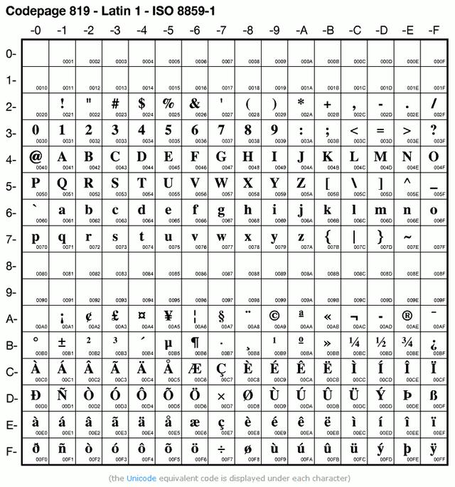
10.4.3 Problems with Single-Byte Encoding
Single-byte (8-bit) encoding, while an improvement over ASCII, still has its own set of problems.
- Inconsistency
- There are a large number of overlapping character sets used for encoding characters in different (European) languages.
- There can be cases where more than one symbol maps to the same code point or number, leading to ambiguity.
- Compatibility
- While it is an improvement over ASCII, it still cannot deal with writing systems with large character sets, such as the CJK (Chinese, Japanese, Korean) languages.
10.4.4 From Single-Byte to Multi-Byte Encoding
- Two-byte character sets
- To address these limitations, two-byte character sets were introduced.
- These sets can represent up to 65,536 (216 = 65536) distinct characters, making them suitable for languages with larger character sets.
- Multiple byte encoding
- Another approach to encoding characters is multiple byte encoding, which is used for languages such as traditional Chinese (Big-5 encoding) and simplified Chinese (GB encoding).
- In these encoding schemes, multiple bytes are used to represent a single character, allowing for a larger set of characters to be encoded.
10.4.5 Problems with Multi-byte Encoding
Different languages still use different encodings, and some are single-byte, while some are multiple-byte. However, digital texts usually have many writing systems at the same time, including single-byte texts, letters, spaces, punctuations, Arabic numerals, interspersed with 2-byte Chinese characters.
- Ambiguity: The inconsistency in the byte-encoding number creates a problem as different languages may use different numbers of bytes to encode the same character, making it challenging to convert between them accurately. This inconsistency creates confusion and ambiguity in the way that text is displayed across different languages.
- Efficiency: Multiple-byte encoding requires a fixed number of bytes for each character, which can result in wasted space when representing characters that require fewer bytes (e.g., ASCII characters). The fixed-length encoding scheme of multiple byte encodings reduces efficiency in terms of storage and transmission.
- Limited character set: Multiple byte encodings often have a limited character set, which means they cannot represent all characters. This limitation makes it difficult to handle text in different languages that utilize non-ASCII characters. It restricts the ability to support a diverse range of languages and writing systems.
10.4.6 Unicode and UTF-8
The objective of modern character encoding is to eliminate the ambiguity of different character sets by specifying a Universal Character Set that includes over 100,000 distinct coded characters, used in all common writing systems today. One of the most widely used character encoding systems is UTF-8.
UTF-8 uses a variable-length encoding system, where each character is coded using one to four bytes. ASCII characters require only one byte in UTF-8 (0-127), ISO-8859 characters require two bytes (128-2,047), CKJ characters require three bytes (2,048-65,535), and rare characters require four bytes (65,536-1,112,064).
UTF-8 has many strengths, including the ability to encode text in any language, the ability to encode characters in a variable-length character encoding, and the ability to encode characters with no overlap or confusion between conflicting byte ranges. UTF-8 is now the standard encoding used for web pages, XML, and JSON data transmission.
10.4.7 Suggestions
- It is always recommended to use the UTF-8 encoding when creating a new dataset.
- It is important to check the encoding of the dataset to avoid ambiguity in character sets.
- When loading a dataset, it is crucial to specify the encoding of the file to ensure accurate interpretation of characters. Garbled characters are usually an indicator of wrong encoding setting.
- One should be cautious of the default encoding used in applications like MS-Word, MS-Excel, Praat, SPSS, etc., while creating, collecting, or editing a dataset.
- It is essential to note that the default encoding for files in Mac/Linux is UTF-8, while in Windows, it is not. Therefore, Windows users need to be extra careful about the encoding of their files.
If you don’t know the encoding of the text file, you can use uchardet::detect_file_enc() to check the encoding of the file:
[1] "ASCII"[1] "UTF-8"[1] "BIG5"10.4.8 Recap: Character, Code Point, and Hexadecimal Mode
- Character: A minimal unit of text that has semantic value in the language (cf. morpheme vs. grapheme), such as
a,我,é. - Code Point: Any legal numeric value in the character encoding set
- Hexadecimal: A positional system that represents numbers using a base of 16.
In R, there are a few base functions that work with these concepts:
Encoding(): Read or set the declared encodings for a character vectoriconv(): Convert a character vector between encodingsutf8ToInt(): Convert a UTF-8 encoded character to integers (code number in decimals)as.hexamode(): Convert numbers into Hexadecimals
[1] "unknown"## Convert the encoding to UTF-8/Big-5
e2 <- iconv(e1, to = "UTF-8")
Encoding(e2) ## ASCII chars are never marked with a declared encoding[1] "unknown"[1] "Q"[1] 81## Convert code number into hex mode
e1_hex <- as.hexmode(e1_decimal)
e1_hex ## code point in hexadecimal mode of `Q`[1] "51"We can represent characters in UTF-8 code point (hexadecimals) by using the escape "\u....":
[1] "Q"[1] "妇"The following is an example of a Chinese character.
[1] "UTF-8"[1] 33274[1] "81fa"[1] "臺"Exercise 10.1 What is the character of the Unicode code point (hexadecimal) U+20AC? How do you find out the character in R?
Exercise 10.2 What is the Unicode code point (in hexadecimal mode) for the character 我 and 你?
Which character is larger in terms of the code points?
Hexadecimal numerals are widely used by computer system designers and programmers, as they provide a human-friendly representation of binary-coded values. One single byte can encode 256 different characters, whose values may range from 00000000 to 11111111 in binary form. These binary forms can be represented as 00 to FF in hexadecimal.
10.5 Native R Functions for I/O
10.5.1 readLines()
When working with text data, it is common to import text files into R for further data processing. To accomplish this, R provides a base function called readLines(). This function reads a txt file using line breaks as the delimiter and returns the contents of the file as a (character) vector. In other words, each line in the text file is treated as an independent element in the vector.
 [1] "[Alice's Adventures in Wonderland by Lewis Carroll 1865]"
 [2] ""
 [3] "CHAPTER I. Down the Rabbit-Hole"
 [4] ""
 [5] "Alice was beginning to get very tired of sitting by her sister on the"
 [6] "bank, and of having nothing to do: once or twice she had peeped into the"
 [7] "book her sister was reading, but it had no pictures or conversations in"
 [8] "it, 'and what is the use of a book,' thought Alice 'without pictures or"
 [9] "conversation?'"
[10] "" [1] "character"[1] 3331Depending on how you arrange the contents in the text file, you may sometimes get a vector of different types:
- If each paragraph in the text file is a word, you get a word-based vector.
- If each paragraph in the text file is a sentence, you get a sentence-based vector.
- If each paragraph in the text file is a paragraph, you get a paragraph-based vector.
There is another native R function for reading text files–scan(), which is similar to readLines(). However, scan() is a more versatile function that can be used to read in a wider variety of file formats, including numeric data and non-textual data. scan() reads in a text file and returns its contents as a vector of atomic objects (numeric, character, or logical), with the values separated by a specified delimiter (e.g., whitespace or commas). That is, scan() allows for users’ defined delimited (unlike the default line break in readLines()).
In summary, readLines() is best used for reading in text files with a consistent line-by-line structure, while scan() is more flexible and can be used for reading in a wider range of data formats.
Exercise 10.3 Based on the inspection of the vector alice created above, what is the content of each line in the original txt file (demo_data/corp-alice.txt)?
If you need to import text files with specific encoding (e.g., big-5, utf-8, gb, ISO8859-1), the recommended method is as follows:
## Reading a big5 file
infile <- file(description = "demo_data/data-chinese-poem-big5.txt",
               encoding = "big-5") ## file as a connection
text_ch_big5 <- readLines(infile) ## read texts from the connection
close(infile) ## close the connection

writeLines(text_ch_big5)
春 眠 不 覺 曉 , 處 處 聞 啼 鳥 。
夜 來 風 雨 聲 , 花 落 知 多 少 。## Reading a utf-8 file
infile <- file(description = "demo_data/data-chinese-poem-utf8.txt",
encoding = "utf-8")
text_ch_utf8 <- readLines(infile)
close(infile)
writeLines(text_ch_utf8) 春 眠 不 覺 曉 , 處 處 聞 啼 鳥 。
夜 來 風 雨 聲 , 花 落 知 多 少 。## Reading a gb18030 file
infile <- file(description = "demo_data/data-chinese-poem-gb2312.txt",
encoding = "gb2312")
text_ch_gb <- readLines(infile)
close(infile)
writeLines(text_ch_gb) 春 眠 不 觉 晓 , 处 处 闻 啼 鸟 。
夜 来 风 雨 声 , 花 落 知 多 少 。You can play with the following methods of loading the text files into R. Like I said, the above method is always recommended. It seems that the encoding settings within the readlines() or other R-native data loading functions (e.g., scan()) do not always work properly. (This is due to the variation of the operation systems and also the default locale of the OS.)
x <- readLines("demo_data/data-chinese-poem-big5.txt", encoding="big-5")
y <- scan("demo_data/data-chinese-poem-big5.txt", what="c",sep="\n", encoding="big-5")
y1 <- scan("demo_data/data-chinese-poem-big5.txt", what="c",sep="\n", fileEncoding="big-5")

# x <- readLines("demo_data/data-chinese-poem-gb2312.txt", encoding="gb2312")
# y <- scan("demo_data/data-chinese-poem-gb2312.txt", what="c",sep="\n", encoding="gb2312")
# y1 <- scan("demo_data/data-chinese-poem-gb2312.txt", what="c",sep="\n", fileEncoding="gb2312")

## The input texts do not show up properly?
writeLines(x)
writeLines(y)
writeLines(y1)
## convert the input texts into your system default encoding
writeLines(iconv(x, from="big-5",to="utf-8"))
writeLines(iconv(y, from="big-5", to="utf-8"))
10.5.2 writeLines()
After processing the data in R, we often need to save our data in an external file for future reference. For text data, we can use the base function writeLines() to save a character vector. By default, each element will be delimited by a line break after it is exported to the file.
Please note that when you writeLines(), you may also need to pay attention to the default encoding of the output file. This is especially important for Windows users. I think R will use the system default encoding as the expected encoding of the output file.
For Mac, it’s UTF-8, which is perfect. However, for Windows, it is NOT. It depends on your OS language.
Can you try to do the following and check the encoding of the output file?
[1] "UTF-8"## For Mac Users, we can output files in different encodings as follows.
## method1
writeLines(x, con = "output_test_1.txt")
## method2
con <- file(description = "output_test_2.txt", encoding="big-5")
writeLines(x, con)
close(con)
## method3
con <- file(description = "output_test_3.txt", encoding="utf-8")
writeLines(x, con)
close(con)
## For Windows Users, please try the following?
x_big5 <- iconv(x, from="utf-8", to = "big-5")
writeLines(x, con = "output_test_w_1.txt", useBytes = TRUE)
writeLines(x_big5, con = "output_test_w_2.txt", useBytes = TRUE)
## Check encodings
uchardet::detect_file_enc("output_test_1.txt") ## mac1[1] "UTF-8"[1] "BIG5"[1] "UTF-8"[1] "UTF-8"[1] "BIG5"It is said that writeLines() will attempt to re-encode the provided text to the native encoding of the system. This works fine when the system default is UTF-8. But in Windows, the default is NOT UTF-8.
I can’t say I fully understand how the encoding system works with Windows. If you would like to know more about this, please refer to this article: String Encoding and R.
Exercise 10.4 Please describe the meaning of the data processing in the code chunk above: sample(alice[nzchar(alice)],10). What did it do with the vector alice?
Exercise 10.5 The above code is repeated below. How do you re-write the code using the %>% pipe-based syntax with a structure provided below? Your output should be exactly the same as the output produced by the original codes.
library(tidyverse)
alice %>%
... %>%
...
... %>%
... %>%
writeLiens(con="corp-alice-2.txt")
Exercise 10.6 In our demo_data directory, there are three text files in different encodings:
demo_data/chinese_gb2312.txtdemo_data/chinese_big5.txtdemo_data/chinese_utf8.txt
Please figure out ways to load these files into R as vectors properly.
- All three files include the same texts:
[1] "這是中文字串。" "文本也有English Characters。"- The simplified Chinese version (i.e.,
chinese_gb2312.txt)
[1] "这是中文字串。" "文本也有English Characters。"10.6 readr Functions
10.6.1 readr::read_csv()
Another common source of data is a spreadsheet-like tabular file, which corresponds to the data.frame in R. Usually we save these tabular data in a csv file, i.e., a comma-separated file. Although R has its own base functions for csv-files reading (e.g., read.table(), read.csv() etc.), here we will use the more powerful version read_csv() provided in the library of readr:
library(readr)
nobel <- read_csv(file = "demo_data/data-nobel-laureates.csv",
                  locale = locale(encoding="UTF-8"))
nobel
The csv file is in fact a normal plain-text file. Each line consists of a row data, with the columns separated by commas. Sometimes we may receive a data set with other self-defined characters as the delimiter.
Another often-seen case is to use the tab as the delimiter. Files with tab as the delimiter are often with the extension tsv. In readr, we can use read_tsv() to read tsv files.
gender_freq <- read_tsv(file = "demo_data/data-stats-f1-freq.tsv",
                        locale = locale(encoding="UTF-8"))
gender_freq
10.6.2 readr::write_csv()
In readr, we can also export our data frames to external files, using write_csv() or write_tsv().
Exercise 10.7 Load the plain-text csv file demo_data/data-bnc-bigram.csv into a data frame and print the top 20 bigrams in the R console arranged by their frequencies (i.e., bi.freq column).
Exercise 10.8 Following Exercise 10.7, please export the data frame of the top 20 bigrams to an external file, named data-bnc-bigram-10.csv, and save it under your current working directory.
10.7 Directory Operations
When we work with external files, we often need to deal with directories as well. Most importantly, we need to know both the paths and filenames of the external data in order to properly load the data into R.
When we work with external files, it is crucial to deal with directories in addition to the files themselves. It is essential to have knowledge of both the path and filename of the external data to ensure that we can accurately load the data into R.
10.7.1 Working Directory
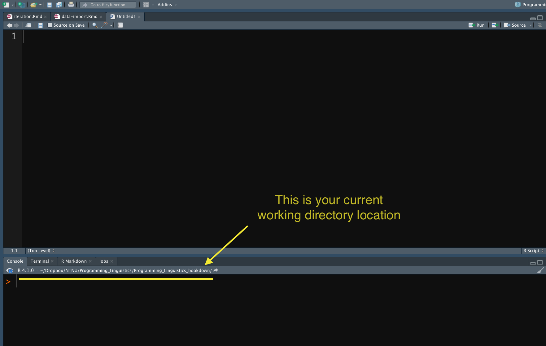
When you start RStudio, R will use a directory as the working directory by default.
- If you start RStudio using the app icon, RStudio will use your system default directory as the working directory.
- If you start RStudio by opening a specific R script, RStudio will use the location of the source file as the working directory.
10.7.2 Relative vs. Absolute Paths
When working with external files in R, we need to specify the path and filename of the external data to load it properly into R. There are two ways to specify the path to an external file, which are the absolute path and the relative path.
The absolute path specifies the complete path to the file location on the computer. This can be very inconvenient as we need to specify the full path every time. For instance, in Windows, the absolute path always starts with the drive label (e.g., C:/Users/Alvinchen/...), while in Mac, it starts with the system root (e.g., /Users/Alvinchen/...).
"C:/Users/Alvin/Documents/ENC2055/demo_data/data-bnc-bigrams.csv"Alternatively, we can use the relative path, which specifies the path in relation to the current working directory. By default, if we only provide the filename, R will search for the file in the working directory. For example, if we use the read_csv("data-bnc-bigram.csv") function, R will look for the file data-bnc-bigram.csv in the working directory. If the file is not in the working directory, R will return an error message.
If the file is located in a sub-directory (of the working directory), we can specify the path to the sub-directory from the current working directory. For instance, read_csv("demo_data/data-bnc-bigram.csv") specifies a sub-directory called demo_data, which is located under the current working directory, and within the sub-directory, R will look for the file data-bnc-bigram.csv.
We can also use .. to specify the parent directory of the current working directory. For example, read_csv("../data-bnc-bigram.csv") specifies that R should look for the file data-bnc-bigram.csv in the parent directory of the current working directory.
It is worth noting that people sometimes use . to refer to the current working directory.
10.7.3 Directory Operations
There are a few important directory operations that we often need when working with files (input/output):
getwd(): check the working directory of the current R sessionsetwd(): set the working directory for the current R session
By default, R looks for the filename or the path under the working directory unless the absolute/relative path to the files/directories is particularly specified.
## get all filenames contained in a directory
dir(path = "demo_data/",
    full.names = FALSE, ## whether to get both filenames & full relative paths
    recursive = FALSE)

## check whether a file/directory exists
file.exists("demo_data/data-bnc-bigram.csv")

## check all filenames contained in the directory
## that goes up two levels from the working dir
dir(path = "../../")
The path dir(path = "../../") specifies a directory path that goes up two levels in the file hierarchy from the current working directory. The double dots .. are used to navigate to the parent directory, so ../ moves up one level in the file hierarchy, and ../../ moves up two levels.
For example, if the current working directory is C:/Users/username/Documents/project/data, then ../../ will take you to C:/Users/username/. If there is a directory named demo at that level, you can access it by appending demo/ to the end of the path: ../../demo/.
10.7.4 Loading files from a directory
When working with external files, it is often necessary to load all the files from a particular directory into R. This task typically involves two steps:
- First, we need to obtain a list of the filenames contained in the directory.
- Next, we need to load the data from each file into R using its corresponding filename.
For example, suppose we want to load all the text files from the directory demo_data/shakespeare. To do this, we need to first obtain a list of the filenames in the directory, and then use a loop to read each file into R based on its filename.
## Corpus root directory
corpus_root_dir <- "demo_data/shakespeare"

## Get the filenames from the directory
flist <- dir(path = corpus_root_dir,
             full.names = TRUE)
flist
[1] "demo_data/shakespeare/Hamlet, Prince of Denmark.txt"
[2] "demo_data/shakespeare/King Lear.txt"
[3] "demo_data/shakespeare/Macbeth.txt"
[4] "demo_data/shakespeare/Othello, the Moor of Venice.txt"## Holder for all data
flist_texts <- list()
## Traverse each file
for (i in 1:length(flist)) {
flist_texts[[i]] <- readLines(flist[i])
}
## peek at first file content
head(flist_texts[[1]]) ## first 6 [1] "< Shakespeare -- HAMLET, PRINCE OF DENMARK >"
[2] "< from Online Library of Liberty (http://oll.libertyfund.org) >"
[3] "< Unicode .txt version by Mike Scott (http://www.lexically.net) >"
[4] "< from \"The Complete Works of William Shakespeare\" >"
[5] "< ed. with a glossary by W.J. Craig M.A. >"
[6] "< (London: Oxford University Press, 1916) >" [1] "</FORTINBRAS>"
[2] "<STAGE DIR>"
[3] "<A dead march. Exeunt, bearing off the bodies; after which a peal of ordnance is shot off.>"
[4] "</STAGE DIR>"
[5] "</SCENE 2>"
[6] "</ACT 5>" In R, we can apply a function to all the elements in a vector using sapply(). We can simplify the code above, which uses a for-loop structure, into one line of code:
## Load data from all files
flist_text <- sapply(flist, readLines)
## peek at first file content
head(flist_texts[[1]]) ## first 6
[1] "< Shakespeare -- HAMLET, PRINCE OF DENMARK >"
[2] "< from Online Library of Liberty (http://oll.libertyfund.org) >"
[3] "< Unicode .txt version by Mike Scott (http://www.lexically.net) >"
[4] "< from \"The Complete Works of William Shakespeare\" >"
[5] "< ed. with a glossary by W.J. Craig M.A. >"
[6] "< (London: Oxford University Press, 1916) >" [1] "</FORTINBRAS>"
[2] "<STAGE DIR>"
[3] "<A dead march. Exeunt, bearing off the bodies; after which a peal of ordnance is shot off.>"
[4] "</STAGE DIR>"
[5] "</SCENE 2>"
[6] "</ACT 5>" Exercise 10.9 Please make yourself familar with the following commands: file.create(), dir.create(), unlink(), basename(),file.info(), save(), and load().
Exercise 10.10 Please create a sub-directory in your working directory, named temp.
Load the dataset demo_data/data-bnc-bigram.csv and subset bigrams whose bigram frequencies (bi.freq column) are larger than 200.
Order the sub data frame according to the bigram frequencies in a descending order and save the sub data frame into a csv file named data-bnc-bigram-freq200.csv in the temp directory.