Chapter 12 Data Scientist First Step
Finally this chapter will demonstrate how you can make use of what you have learned from the previous chapters to perform an exploratory data analysis on the dataset you are interested in. Here we will look at a dataset of Nobel Laureates.
Before you start, always remember to load necessary R libraries first.
12.1 Loading Nobel Laureates Dataset
## Data Import
my_df <- read_csv(file = "demo_data/data-nobel-laureates.csv",
                  locale = locale(encoding="UTF-8"))

## Peek
my_df
When loading the data, R throws an warning message about parsing issues in the file. We can check the issues using the following method:
spc_tbl_ [969 × 18] (S3: spec_tbl_df/tbl_df/tbl/data.frame)
 $ Year                : num [1:969] 1901 1901 1901 1901 1901 ...
 $ Category            : chr [1:969] "Chemistry" "Literature" "Medicine" "Peace" ...
 $ Prize               : chr [1:969] "The Nobel Prize in Chemistry 1901" "The Nobel Prize in Literature 1901" "The Nobel Prize in Physiology or Medicine 1901" "The Nobel Peace Prize 1901" ...
 $ Motivation          : chr [1:969] "\"in recognition of the extraordinary services he has rendered by the discovery of the laws of chemical dynamic"| __truncated__ "\"in special recognition of his poetic composition, which gives evidence of lofty idealism, artistic perfection"| __truncated__ "\"for his work on serum therapy, especially its application against diphtheria, by which he has opened a new ro"| __truncated__ NA ...
 $ Prize Share         : chr [1:969] "1/1" "1/1" "1/1" "1/2" ...
 $ Laureate ID         : num [1:969] 160 569 293 462 463 1 161 571 294 464 ...
 $ Laureate Type       : chr [1:969] "Individual" "Individual" "Individual" "Individual" ...
 $ Full Name           : chr [1:969] "Jacobus Henricus van 't Hoff" "Sully Prudhomme" "Emil Adolf von Behring" "Jean Henry Dunant" ...
 $ Birth Date          : Date[1:969], format: "1852-08-30" "1839-03-16" ...
 $ Birth City          : chr [1:969] "Rotterdam" "Paris" "Hansdorf (Lawice)" "Geneva" ...
 $ Birth Country       : chr [1:969] "Netherlands" "France" "Prussia (Poland)" "Switzerland" ...
 $ Sex                 : chr [1:969] "Male" "Male" "Male" "Male" ...
 $ Organization Name   : chr [1:969] "Berlin University" NA "Marburg University" NA ...
 $ Organization City   : chr [1:969] "Berlin" NA "Marburg" NA ...
 $ Organization Country: chr [1:969] "Germany" NA "Germany" NA ...
 $ Death Date          : Date[1:969], format: "1911-03-01" "1907-09-07" ...
 $ Death City          : chr [1:969] "Berlin" "Châtenay" "Marburg" "Heiden" ...
 $ Death Country       : chr [1:969] "Germany" "France" "Germany" "Switzerland" ...
 - attr(*, "spec")=
  .. cols(
  ..   Year = col_double(),
  ..   Category = col_character(),
  ..   Prize = col_character(),
  ..   Motivation = col_character(),
  ..   `Prize Share` = col_character(),
  ..   `Laureate ID` = col_double(),
  ..   `Laureate Type` = col_character(),
  ..   `Full Name` = col_character(),
  ..   `Birth Date` = col_date(format = ""),
  ..   `Birth City` = col_character(),
  ..   `Birth Country` = col_character(),
  ..   Sex = col_character(),
  ..   `Organization Name` = col_character(),
  ..   `Organization City` = col_character(),
  ..   `Organization Country` = col_character(),
  ..   `Death Date` = col_date(format = ""),
  ..   `Death City` = col_character(),
  ..   `Death Country` = col_character()
  .. )
- attr(*, "problems")=<externalptr> Year Category Prize Motivation
Min. :1901 Length:969 Length:969 Length:969
1st Qu.:1947 Class :character Class :character Class :character
Median :1976 Mode :character Mode :character Mode :character
Mean :1970
3rd Qu.:1999
Max. :2016
Prize Share Laureate ID Laureate Type Full Name
Length:969 Min. : 1.0 Length:969 Length:969
Class :character 1st Qu.:230.0 Class :character Class :character
Mode :character Median :462.0 Mode :character Mode :character
Mean :470.2
3rd Qu.:718.0
Max. :937.0
Birth Date Birth City Birth Country Sex
Min. :1817-11-30 Length:969 Length:969 Length:969
1st Qu.:1891-06-02 Class :character Class :character Class :character
Median :1916-09-14 Mode :character Mode :character Mode :character
Mean :1911-02-02
3rd Qu.:1935-07-13
Max. :1997-07-12
NA's :31
Organization Name Organization City Organization Country
Length:969 Length:969 Length:969
Class :character Class :character Class :character
Mode :character Mode :character Mode :character
Death Date Death City Death Country
Min. :1903-11-01 Length:969 Length:969
1st Qu.:1954-07-14 Class :character Class :character
Median :1980-04-15 Mode :character Mode :character
Mean :1975-03-04
3rd Qu.:1999-07-26
Max. :2017-02-08
NA's :352 When dealing with files that contain Chinese or non-English characters, or files encoded in UTF-8, I recommend explicitly specifying the encoding of the file to ensure proper data import.
12.3 Column Names
Before we begin, it’s evident that the column names contain spaces that we want to remove. Our objective is to eliminate the spaces and replace them with underscores (_).
 [1] "Year"                 "Category"             "Prize"
 [4] "Motivation"           "Prize Share"          "Laureate ID"
 [7] "Laureate Type"        "Full Name"            "Birth Date"
[10] "Birth City"           "Birth Country"        "Sex"
[13] "Organization Name"    "Organization City"    "Organization Country"
[16] "Death Date"           "Death City"           "Death Country"
## Overwrite the original with new ones
names(my_df) <- str_replace_all(names(my_df), "\\s","_")
## Autoprint updated my_df
my_df [1] "Year" "Category" "Prize"
[4] "Motivation" "Prize_Share" "Laureate_ID"
[7] "Laureate_Type" "Full_Name" "Birth_Date"
[10] "Birth_City" "Birth_Country" "Sex"
[13] "Organization_Name" "Organization_City" "Organization_Country"
[16] "Death_Date" "Death_City" "Death_Country" By completing these steps, we will have transformed the column names by removing spaces and replacing them with underscores, ensuring consistency and ease of use in further data processing.
12.4 Missing Data (NA values)
It is always important to check if the information of each row is complete.
- We first define a function
check_num_NA(), which checks the number ofNAvalues of the inputxobject - We then
map()this self-defined function to each column of themy_df
## Define a custom function
check_num_NA <- function(x){
  sum(is.na(x))
}

## Map the function to the data frame
my_df %>% map_df(check_num_NA) Year Category Prize
0 0 0
Motivation Prize_Share Laureate_ID
88 0 0
Laureate_Type Full_Name Birth_Date
0 0 31
Birth_City Birth_Country Sex
28 26 26
Organization_Name Organization_City Organization_Country
247 253 253
Death_Date Death_City Death_Country
352 370 364 ## Alternatively, you can write this way:
# map_df(my_df, check_num_NA)
# map_int(my_df, check_num_NA)From the above results, we see that Sex column has 26 cases of NA values.
We can examine the rows with NA’s in more detail by filtering out these cases:
After inspection of these 26 cases, can you make any generalization to account for their missing values in Sex column?
Another method is to examine cases/rows where there is at least one NA value, using complete.cases():
[1] 0.5614035When dealing with NA (missing) values in data analysis, here are a few suggestions to consider:
Identify the presence of NA values: Begin by checking your data to identify the presence of NA values. This can be done using functions like
is.na()orcomplete.cases().Understand the nature of missingness: It’s essential to understand why the NA values exist in your data. Are they at random or systematic? This understanding can help inform the appropriate handling strategy.
Analyze missing data patterns: It can be insightful to analyze the patterns and relationships between missing values and other variables. This analysis can provide additional insights into the reasons for missingness and potential biases in your data.
Remove NA values: In some cases, you may choose to remove rows or columns with NA values if they are not critical for your analysis. This can be done using functions like
na.omit()orcomplete.cases().Impute missing values: If the NA values are significant and removing them would result in a loss of valuable information, you can impute (replace) them with estimated values. Common imputation methods include mean imputation, median imputation, or using more advanced techniques like regression imputation or multiple imputation.
Document and report missing data handling: Whichever approach you choose, it’s important to document and report how you handled missing data. This ensures transparency and allows others to understand the impact of missing data on your analysis.
12.5 Data Preprocessing
Before proceeding with data analysis, it is essential to preprocess the data to make sure that it is appropriately prepared for your later quantitative (statistical) analysis.
In a real-world dataset, it is often to encounter duplicate data points (e.g., Laureate_ID = 838):
Alternatively, the factor of interest may be implicit and embedded within the dataset. For example, if we would like to examine the Nobel Prize winners by “the age of winning” or “the decades”, these factors of interest may not be straightforward from the existing columns in the dataset:
## Check `Year` and `Bird_Date`
## Information implicit in these columns
my_df %>%
  select(Laureate_ID, Year, Full_Name, Birth_Date, Category)
Some common considerations for data preprocessing include:
- ✅ Cleaning the column names to ensure they are consistent and easy to work with.
- ✅ Handling missing data
- Creating unique indices for all data points
- Lowercasing all character vectors (i.e., text columns) to normalize the letter casing
- Identifying duplicate tokens within the dataset
- Creating new columns that better reflect the factors of interest, such as:
DecadePrize_Age
## Data preprocessing
nobel_winners <- my_df %>%
  mutate(id = row_number()) %>% ## unique row indices
  mutate_if(is.character, tolower) %>% ## lower all character vectors
  distinct_at(vars(Full_Name, Year, Category), .keep_all = TRUE) %>% ## duplicates
  mutate(Decade = 10 * (Year %/% 10), ## create new factors
         Prize_Age = Year - lubridate::year(Birth_Date))

## check
nobel_winners
Please note that the necessity of the aforementioned preprocessing steps may vary depending on the characteristics of your dataset and the specific research questions you are addressing. It is important to carefully consider which preprocessing steps are relevant and applicable to your particular case.
Furthermore, the order in which these preprocessing steps are performed is not arbitrary and can have an impact on the outcomes of your analysis. The optimal ordering of preprocessing steps may vary depending on the nature of your data and the objectives of your research. It is advisable to take into account the specific requirements and considerations of your study when determining the most appropriate order for performing these steps.
Given two positive integers, normally, we define the division as follows: a / b in R.
There are two variants of the integer division:
a %% b(a modulo b): This modulo operation will return the remainder of the division (The expression5 %% 3would evaluate to2).a %/% b: This integer division operation will return the quotient of the division (The expression5 %/% 3would evaluate to1).
We often use this modulo operation to check if an output value is a multiple of a specific integer.
We can check if our new Prize_Age has any NA values?
nobel_winners %>%
  filter(is.na(Prize_Age)) %>%
  select(Laureate_ID, Year, Full_Name, Birth_Date, Prize_Age)
Check Chinese laureates again:
nobel_winners %>%
  filter(Birth_Country == "china") %>%
  select(Laureate_ID, Full_Name, Year, Category)
12.6 Exploratory Analysis
After performing data preprocessing, the next step is to conduct exploratory data analysis. As mentioned in Chapter 7, data visualization is often a useful starting point for exploratory analysis.
In this section, we will explore how to generate relevant statistics and graphs based on different research questions. By utilizing these tools, we can gain insights and uncover patterns in the data, helping us better understand the underlying relationships and trends.
12.6.1 Discipline Distribution
- RQ: What is the distribution of laureates across different disciplines?
## barplots
nobel_winners %>%
  count(Category) %>%
  ggplot(aes(x = Category, y = n, fill = Category)) +
  geom_col() +
  geom_text(aes(label = n), vjust = -0.25) +
  labs(title = "No. of Laureates in Different Disciplines", x = "Category", y = "N") +
  theme(legend.position = "none")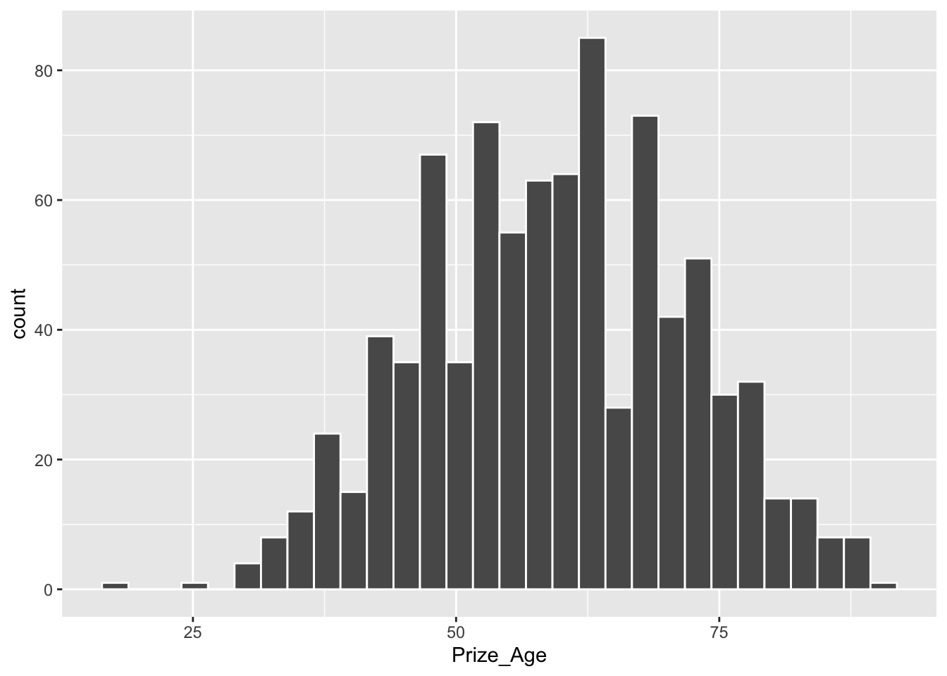
## barplots (ordered)
nobel_winners %>%
  count(Category) %>%
  ggplot(aes(x = fct_reorder(Category, -n), y = n, fill = Category)) +
  geom_col() +
  geom_text(aes(label = n), vjust = -0.25) +
  labs(title = "No. of Laureates in Different Disciplines", x = "Category", y = "N") +
  theme(legend.position = "none")
An even more dynamic graph:
## barplot (dynamic)

## Uncomment if you have not installed this library
# install.packages("gganimate", dependencies = T)
library(gganimate)

my_df %>%
  count(Category) %>%
  mutate(Category = fct_reorder(Category, -n)) %>%
  ggplot(aes(x = Category, y = n, fill = Category)) +
  geom_text(aes(label = n), vjust = -0.25) +
  geom_col()+
  labs(title = "No. of Laureates in Different Disciplines", x = "Category", y = "N") +
  theme(legend.position = "none") +
  transition_states(Category)  +
  shadow_mark(past = TRUE)
12.6.2 Age Distribution
- RQ: At what age did laureates normally win their Nobel Prizes?
   Min. 1st Qu.  Median    Mean 3rd Qu.    Max.    NA's
17.00 50.00 60.00 59.45 69.00 90.00 30 X1
vars 1.00000000
n 881.00000000
mean 59.45175936
sd 12.41297890
median 60.00000000
trimmed 59.50496454
mad 13.34340000
min 17.00000000
max 90.00000000
range 73.00000000
skew -0.04907038
kurtosis -0.44875709
se 0.41820389## histogram
nobel_winners %>%
filter(!is.na(Prize_Age)) %>%
ggplot(aes(x = Prize_Age)) +
geom_histogram(color="white")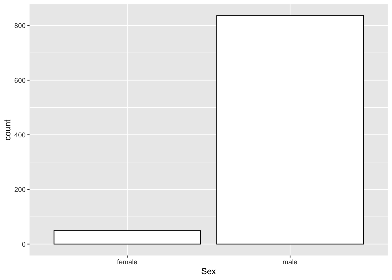
## boxplot
nobel_winners %>%
  filter(!is.na(Prize_Age)) %>%
  ggplot(aes(y = Prize_Age)) +
  geom_boxplot()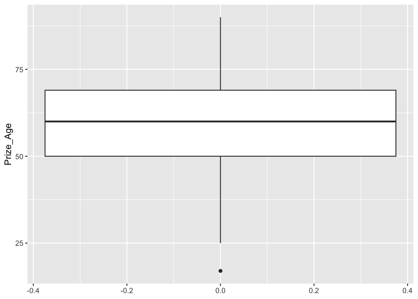
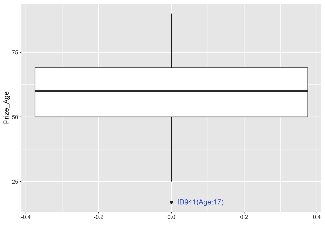
Exercise 12.1 In the above example, we can see that in the boxplot, there is one outlier in terms of the prize winning age. How can we identify this particular case from the dataset and specify its information (i.e., id and prize_age) in the graph?
12.6.3 Category x Age Interaction
- RQ: Is there variation in the age of prize winners across different prize categories?
## Statistics
nobel_winners %>%
  filter(!is.na(Prize_Age)) %>%
  group_by(Category) %>%
  summarize(mean_age = mean(Prize_Age),
            sd_age = sd(Prize_Age)) %>%
  ungroup %>%
  arrange(mean_age)
## Histogram
nobel_winners %>%
filter(!is.na(Prize_Age)) %>%
ggplot(aes(x = Prize_Age, fill = Category, color = Category)) +
geom_histogram(color="white") +
facet_wrap(~Category) +
theme(legend.position = "none")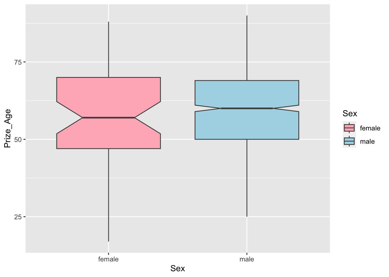
## Density graphs
nobel_winners %>%
  filter(!is.na(Prize_Age)) %>%
  ggplot(aes(x = Prize_Age, fill = Category, color = Category))  +
  geom_density() +
  facet_wrap(~Category) +
  theme(legend.position = "none")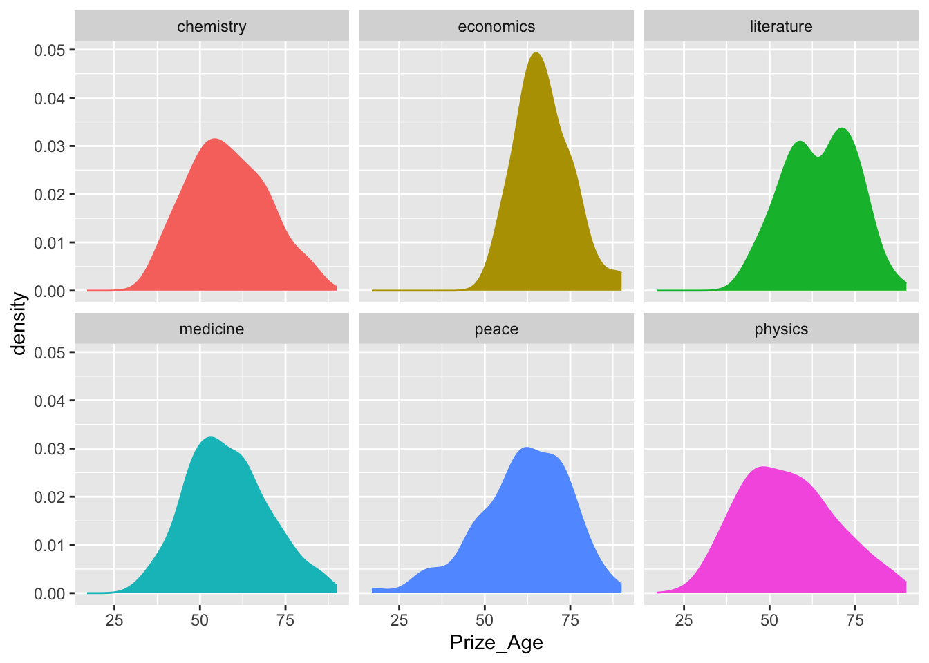
## boxplot
nobel_winners %>%
  filter(!is.na(Prize_Age)) %>%
  ggplot(aes(x = Category, y = Prize_Age, fill = Category))+
  geom_boxplot(notch=T)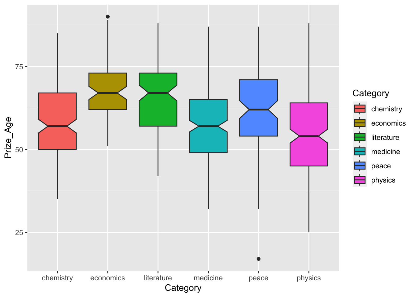
## mean and CI plots
nobel_winners %>%
  filter(!is.na(Prize_Age)) %>%
  ggplot(aes(Category, Prize_Age, fill = Category)) +
  stat_summary(fun = mean, geom = "bar", fill="white", color="black") +
  stat_summary(fun.data = function(x) mean_se(x, mult = 1.96),
               geom = "errorbar", width = 0.1, color="grey40")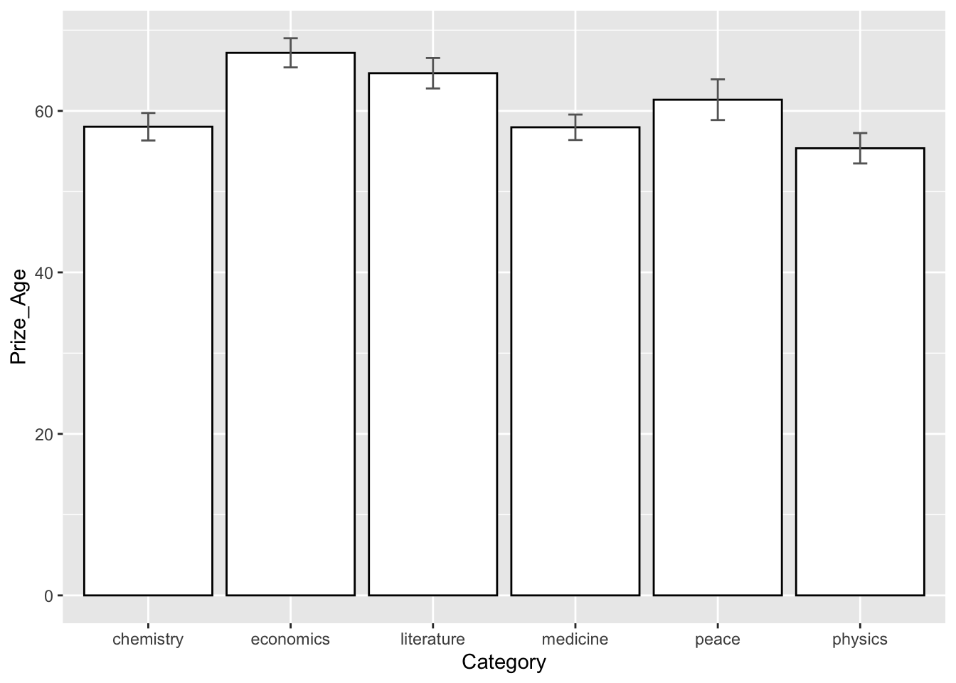
geom_density_ridges() is a visualization function from the ggridges package in R. It allows you to create ridgeline plots, also known as density ridgeline plots or joyplots. These plots display the density distribution of a variable across different categories or groups.
The function geom_density_ridges() takes your data and maps a continuous variable to the y-axis to represent the density. The x-axis represents the categories or groups you want to compare. Each category is represented by a ridgeline, and the density of the variable is visualized as the height or thickness of the ridgeline.
This visualization is useful for comparing the distributions of a continuous variable across different groups, as it provides a clear and compact representation of the density curves for each group. It allows you to identify variations in the density and explore patterns or differences between groups in a visually appealing manner.
library(ggridges)

nobel_winners %>%
  filter(!is.na(Prize_Age)) %>%
  ggplot(aes(x = Prize_Age,
             y = Category,
             fill = Category)) +
  geom_density_ridges()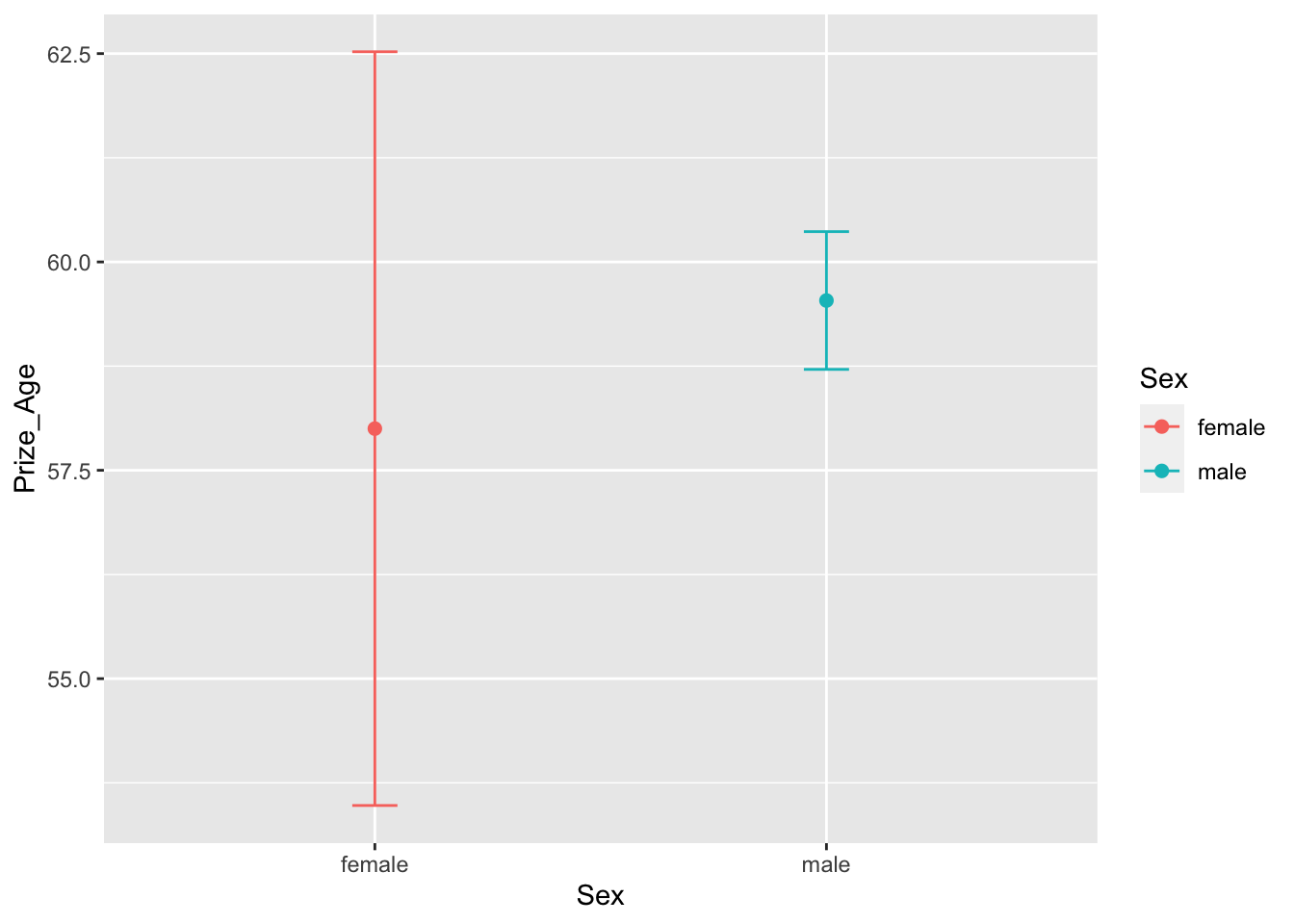
12.6.4 Gender Distribution
- RQ: What is the gender distribution of Nobel winners?
## statistics
nobel_winners %>%
  filter(!is.na(Sex)) %>%
  count(Sex) %>%
  mutate(percent = round(n/sum(n),2))
## graphs
nobel_winners %>%
filter(!is.na(Sex)) %>%
ggplot(aes(Sex)) +
geom_bar(fill="white",color="black") 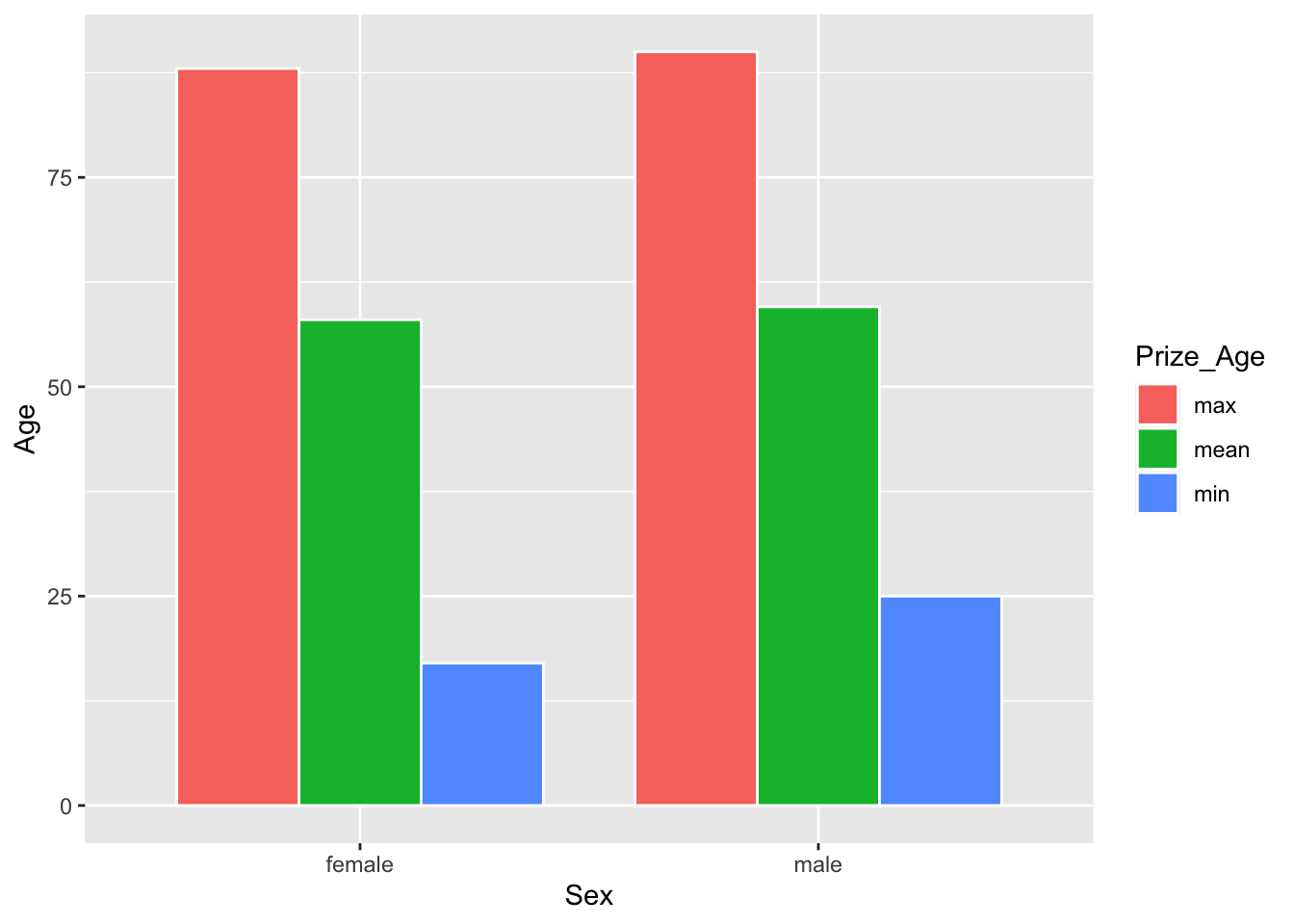
12.6.5 Age x Gender Interaction
- RQ: Did the ages differ greatly for male and female winners?
## statistics
nobel_winners %>%
  filter(!is.na(Sex) & !is.na(Prize_Age)) %>%
  group_by(Sex) %>%
  summarize(mean_prize_age = mean(Prize_Age),
            sd_prize_age = sd(Prize_Age),
            min_prize_age = min(Prize_Age),
            max_prize_age = max(Prize_Age),
            N = n()) -> sum_sex_age

## Check
sum_sex_age
As for visualization, we can create boxplots for male and female winners.
## boxplot
nobel_winners %>%
  filter(!is.na(Sex) & !is.na(Prize_Age)) %>%
  ggplot(aes(Sex, Prize_Age, fill=Sex)) +
  geom_boxplot(notch=T, color="grey30") +
  scale_fill_manual(values = c("lightpink","lightblue"))
Or alternatively, we can create the mean and confidence interval plots for winner’s age distribution for each gender.
## Mean and CI Plot
## you have to have this for `stat_summary()`
# require(Hmisc)
nobel_winners %>%
  filter(!is.na(Sex) & !is.na(Prize_Age)) %>%
  ggplot(aes(Sex, Prize_Age, color=Sex)) +
  stat_summary(fun = mean, geom = "point", size = 2) +
  stat_summary(fun.data = function(x) mean_se(x, mult=1.96),
               geom = "errorbar",
               width = 0.1)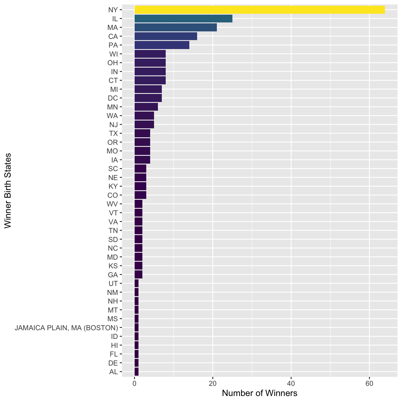
We can create an informative graph showing not only the mean ages of male and female winners, but also their respective minimum and maximum ages.
## Barplot
sum_sex_age %>%
  pivot_longer(cols = c("mean_prize_age","min_prize_age", "max_prize_age"),
               names_to = "Prize_Age",
               values_to = "Age") %>%
  mutate(Prize_Age = str_replace_all(Prize_Age, "_prize_age$","")) %>%
  ggplot(aes(Sex, Age, fill=Prize_Age)) +
  geom_bar(stat="identity",
           width = 0.8,
           color="white",
           position = position_dodge(0.8))
12.6.6 State Distribution
- RQ: What is the distribution of Nobel Prize winners’ states for American laureates?
We can explore the state distribution of the US Nobel Winners. This would give us an idea which state in the United States has the most Nobel winners.
To start with, for US winners, we can extract their birth states from their birth cities (using regular expressions of course):
## Explore the data
nobel_winners %>%
  filter(Birth_Country == "united states of america") %>%
  select(Year, Category, Full_Name, Birth_City)
Now we can utilize regular expression to extract the state from the birth cities:
nobel_winners %>%
  filter(Birth_Country == "united states of america") %>%
  mutate(Birth_State = str_replace(Birth_City, "([^,]+), ([a-z]+)$", "\\2")) %>%
  group_by(Birth_State) %>%
  summarize(N = n()) %>%
  arrange(desc(N), Birth_State) -> sum_state

sum_state
And then we can plot the US winner’s state distribution:
sum_state %>%
  mutate(Birth_State = fct_reorder(str_to_upper(Birth_State), N)) %>%
  ggplot(aes(Birth_State, N, fill = N)) +
  geom_col() +
  coord_flip() +
  scale_fill_viridis_c(guide=F) +
  labs(y = "Number of Winners", x = "Winner Birth States")
In the above bar plot, we can see that there is one false positive (e.g., JAMAICA PLAIN, MA (BOSTON)) in the matches of the regular expression. How can we adjust the regular expression to fix this issue?
In the demo-data/US-states-csv, you can find a csv with the mapping between states abbreviations and their full names. We can include the full names of states in the above result by adding another column.
- The
US-states.csvdataset
## Joining tables
sum_state %>%
mutate(Birth_State = str_to_upper(Birth_State)) %>%
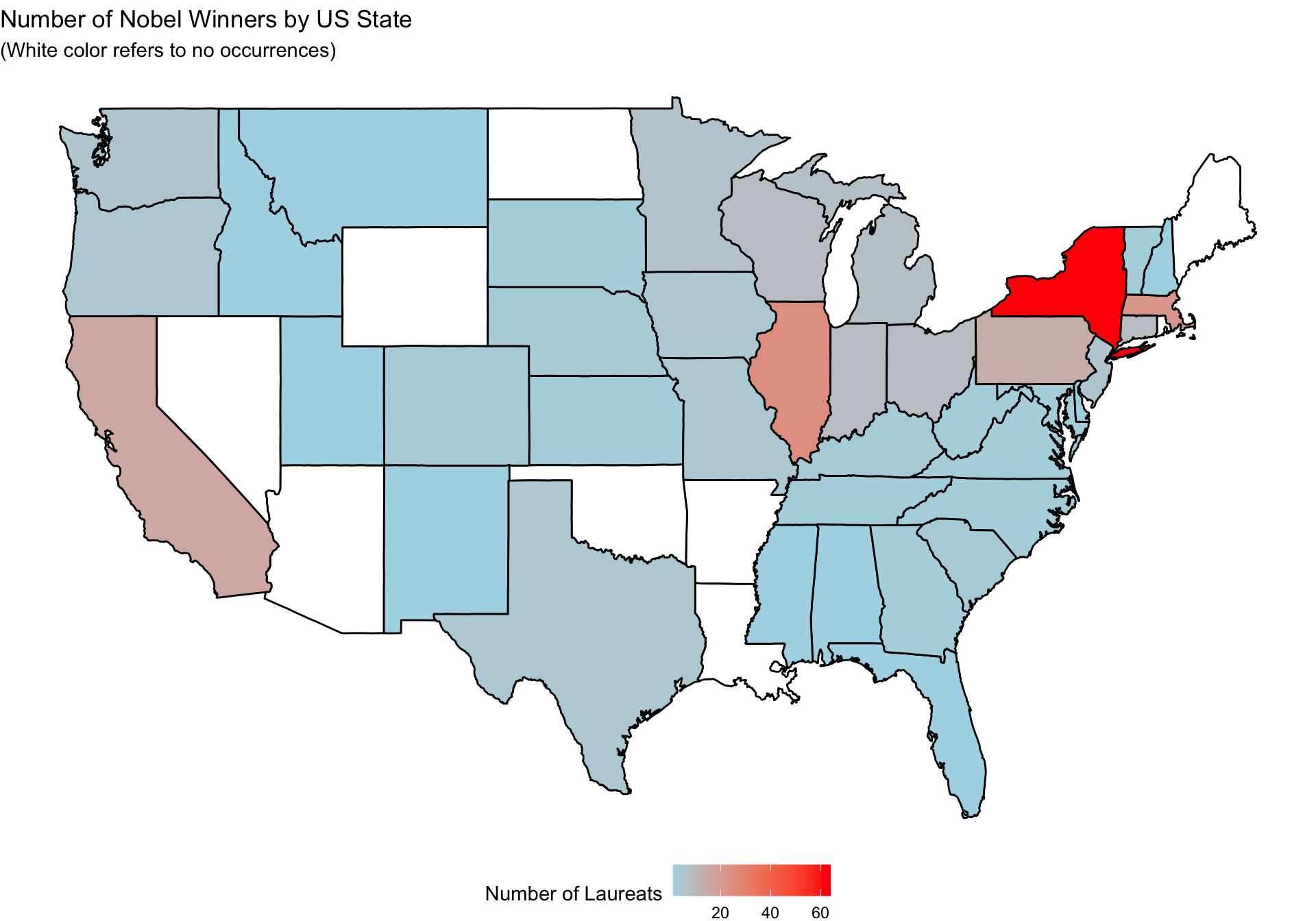
left_join(US_states, by = c("Birth_State" = "Code"))Exercise 12.2 Please create a map of the United States that shows the number of laureates in each state, with states colored according to their respective number of laureates.
12.7 Exercises
Exercise 12.3 Create a subset of nobel_winners, which includes only winners who won the prizes more than once and in more than one category.
Exercise 12.4 Please create a data frame of summary statistics, which shows us the distributions of male and female winners in different categories as shown below. Also, please show the number of males and females as well as the proportions for each prize category. (i.e., frequencies and normalized frequencies)
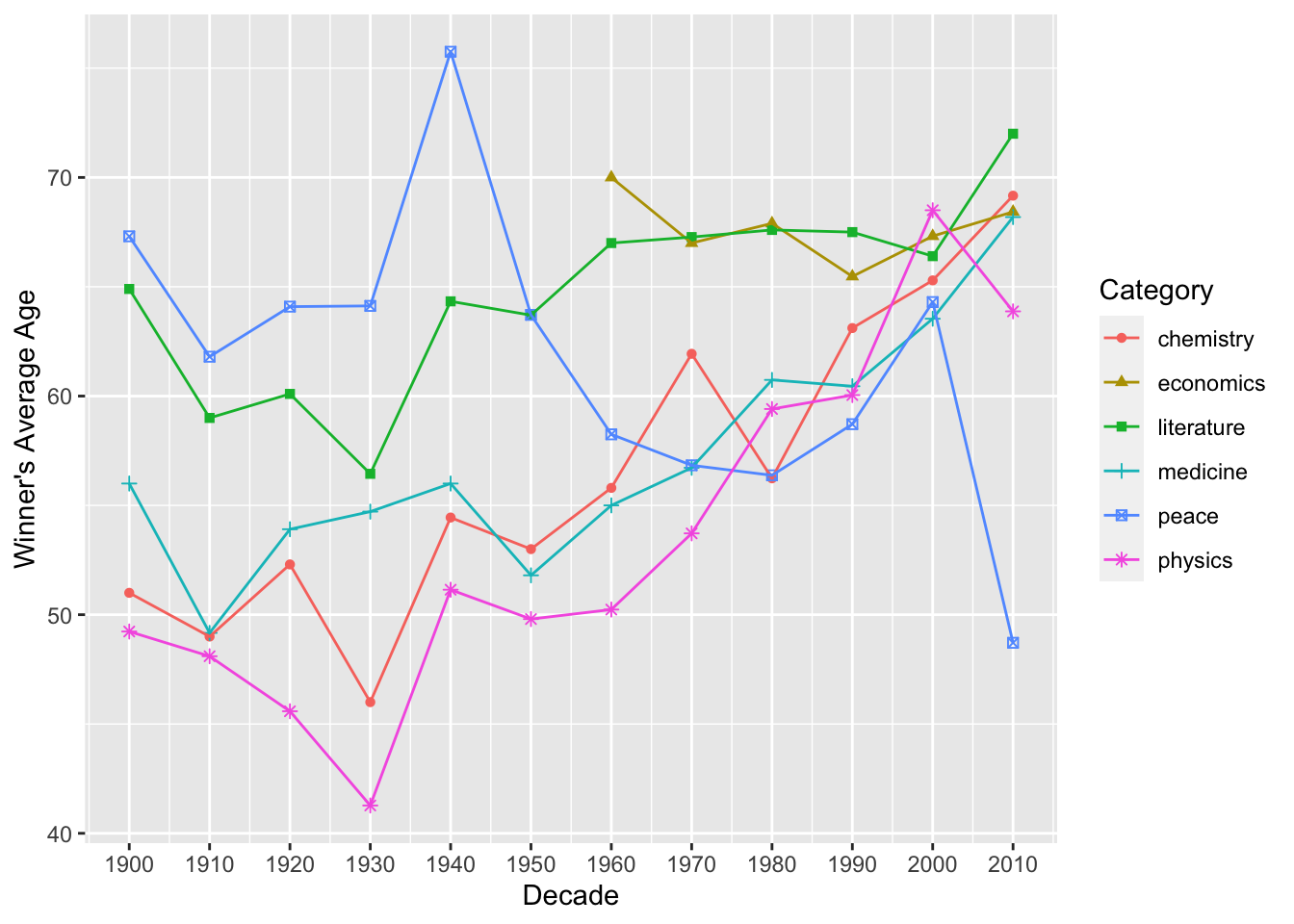
Exercise 12.5 Create a line plot that illustrates the average ages of prize winners for different categories over different decades.