Chapter 6 Functions

We have been using R functions in the default base R package, such as c(), list(), sample(). R provides a lot of useful built-in functions like these, but we can write our own task-specific functions as well. A function is like a mini-program within a program. In this unit, we discuss how to write functions in R.

6.1 A Quick Start

To better understand how a function works, let’s create a simple one. The following code chunk creates a function object, named hello().

hello <- function() {
    print("How are you doing?")
}

A function object includes several important elements:

We use the function() keyword to define a new function object.
After the function() keyword is the code block ({...}), which contains the body of the function. That is, the code block is the set of instructions that perform the desired task.
The body of the function function(Parameter1, Parameter2, ...) can take arguments (inputs) that are passed to the function when it is called (See next section.)
Every function is assigned to a user-defined name (e.g., hello in the above example.)

Once a function is defined using the function() keyword in R, the code within the body of the function will not be executed immediately.

Rather, the code will only be executed when the function is called. Whenever the function is called, it will execute the code within its body, carrying out the specific tasks defined in the function’s code block.

This allows for code reuse and modularity, as the same code can be called multiple times with different inputs, rather than having to rewrite the same code multiple times.

hello()

[1] "How are you doing?"

hello()

[1] "How are you doing?"

6.2 Why do we need functions?

A major advantage of creating functions in our programs is to group codes that get executed multiple times. Without a function defined, one may need to copy-and-paste same code chunks many times.

Second, with functions, it is easier to update the programs. We often try to avoid duplicating code because if we need to update the code (e.g., to fix a bug in the original code), we don’t have to change the code everywhere we have copied it.

In short, functions can greatly reduce the chances of duplicating code, rendering the programs shorter, easier to read and update.

6.3 Functions with parameters

When we use the built-in R functions like cat(), length(), or matrix(), we can pass them values, called arguments, in the parentheses.

That is, some functions have parameters and users can pass values to each parameter as arguments.

In our self-defined functions, we can also define a function which accepts arguments.

hello <- function(name) {
    cat("How are you doing,", name)
}

hello(name = "Alvin")

How are you doing, Alvin

The new hello() function has a parameter called name. Parameters are variables that expect arguments in the function call. When a function is called with an argument (e.g., Alvin), this argument is stored in the parameter (e.g., name).

More specifically, when the function hello(name = 'Alvin') is called:

The argument "Alvin" is assigned to the parameter name;
The program then continues the code block of the function;
Within the code block, the parameter name is automatically set to Alvin.

It is important to note that the value stored in the parameter is forgotten when the function returns. That is, we cannot access the parameter name in the main program:

cat(name)

Error in cat(name): object 'name' not found

In short, the parameters of a function are destroyed after a function call hello(name = 'Alvin') returns.

In the function definition, we can specify default values to the parameters. For example, if the function hello() is defined as follows, users can decide whether to accept the default argument or assign the parameter name with a new argument:

hello <- function(name = "Alvin") {
    cat("How are you doing,", name)
}

## call 1
hello()

How are you doing, Alvin

## call 2
hello(name = "Superman")

How are you doing, Superman

6.4 Recap of Important Concepts So Far

To utilize a function object, there are several key steps:

We need to define the function by creating it using hello <- function(){...} and assigning it with an object name like any other objects in R.
Then we can call the now-created function using hello().
The function call will start the execution of the code block in the function by first passing or assigning the arguments/values to the parameters within the function (e.g., hello(name = 'Alvin')).
- A value being passed to a function in a function call is an argument, (e.g., Alvin)
- Variables that have arguments assigned to them are parameters, (e.g., name =).

6.5 RETURN Statements

When we define a function, we can specify what the return values should be using the return() statement.

The returned values, i.e., the output object of the function, can then be assigned to a new object name for later use in the program.

In R, there are many built-in functions that return values:

num <- sample(1:10, 3)
num

[1] 3 5 8

When a function returns nothing, by default the return value of the function is NULL, which is a unique data type in R referring to NoneType.

out <- cat("This is a sentence")  # `cat()` has no return

This is a sentence

out

NULL

Now how about the hello() function we created earlier? We didn’t specify the return() statement in the function definition.

out <- hello(name = "John")

How are you doing, John

out

NULL

In the definition of hello(), we did not specify the return() statement; therefore, by default, this function returns NULL. But how come we can still see the outputs of the function?

In the code block of hello() definition, the cat() displays text on the R console only. Therefore, displaying texts in the R console and returning the values are two different things.

Exercise 6.1 The function hello() prints a message to the console. Without any change of the function definition hello(), how can we capture the messages printed in the console by hello() and save them to an object named out?

Your task is to modify the following code chunk so that out can store the messages printed by hello(name="Alvin"). Keep in mind that you cannot modify the definition of hello() itself, so you will need to use a different approach to capture its output.

out <- hello(name="Alvin")
out

Exercise 6.2 Can you try to create a revised version of hello(), which returns the strings so that one can assign the outputs of the hello() to another object name? (Please note that in the following example, the return value out is not a NULL anymore.)

out <- hello2(name = "Alvin")
out

[1] "How are you doing, Alvin"

hello2(name = "John")

[1] "How are you doing, John"

6.6 Parameters Order

We’ve seen functions with parameters. When a function has many parameters, there are two alternatives to assign the arguments to the parameters in the function call.

First, we can assign the arguments to the parameters specified in the function call:

set.seed(123)
sample(x = c(1:10), size = 5, replace = FALSE, prob = NULL)

[1]  3 10  2  8  6

Alternatively, we can assign the arguments to the parameters according to the order of the parameters in th function definition without specifying the parameter names:

set.seed(123)
sample(c(1:10), 5, FALSE, NULL)

[1]  3 10  2  8  6

In the function definition, we can also assign default values to the parameters. For example, in the documentation of sample(x, size, replace = FALSE, prob = NULL), we can see that the parameters replace= and prob= have default values. That means in the function call we can use these default values as the arguments without specifying them in the call.

sample(c(1:10), 5)

[1] 5 4 6 8 1

6.7 Stacking Functions

A function can also call another function within its code block. When this happens, the execution of the code would move to the called function before returning to the original function call.

For instance, we can define two functions in R, hello() and email().

## Main function
hello <- function(name) {
    user_email <- email(user = name)
    out <- paste0("How are you doing, ", name, ". ", user_email)

    return(out)
}

## Embedded function
email <- function(user) {
    out <- paste0("Your email is: ", tolower(user), "@whatever.org")
    return(out)
}

Within the code block of hello(), we can make a function call to email(). This means that email() is embedded within hello(), and when hello() is called, it will execute its code block and then move to execute the code block of email(). After the code block of email() is executed, the control will move back to hello() to complete its execution.

## call `hello()`
hello("Alvin")

[1] "How are you doing, Alvin. Your email is: alvin@whatever.org"

This ability to call functions within functions is useful in situations where a function needs to perform multiple tasks, and each task can be implemented using a separate function. Rather than writing all the code in a single function, we can call other functions from within it to keep the code organized and easier to understand.

6.8 Local and Global Scope

Now we know that functions allow us to organize code into reusable blocks that perform specific tasks. We only have to write code once and can call it multiple times with different inputs.

When we call a function, it creates its own workspace or environment, called the local scope. Any variables created or modified inside the function only exist within that function and are known as local variables. These variables cannot be accessed or modified outside of the function.

On the other hand, variables that are created outside of any functions are said to exist in the global scope. These variables are known as global variables and are accessible to all functions and code blocks in the program. Any changes made to global variables inside a function will affect the global variable’s value outside the function.

A scope is like the life-span of the variable. A local scope is created whenever a function is called. Any variables created in the function exist within the function’s local scope. When the function returns, the local scope is destroyed, and these local variables are forgotten (i.e., removed from the memory of the current working environment).

The global scope is created when the main program starts (e.g., your current R session). When the program terminates, the global scope is destroyed, and all the global variables are forgotten.

There are a few important considerations for variable scope:

Code in the global scope (i.e., outside of all functions) cannot use any local variables (i.e., variables within functions).
Code in a local scope can access global variables.
Code in a local scope can modify the values of global variables.
Code in a function’s local scope cannot use variables in any other local scope.
We can use the same name for different variables if they are in different scopes (e.g., they can be local variables within different functions).

While using global variables within functions in small programs may not cause significant issues, it is generally considered bad practice to rely on global variables in larger programs.

One issue with using global variables in local functions is that they can be accessed and modified by any part of the program, making it difficult to track changes and debug the code.

Another issue is that global variables can make it difficult to reuse functions in other parts of the program or in other programs.

In short, functions that rely on global variables are less modular and less portable, and can make code maintenance and updates more difficult in the long run.

The following code chunk shows that local variables cannot be accessed in the global scope.

customer <- function() {
    id <- 123
    age <- 25
    nation <- "TW"
}
customer()
cat(id)

Error in cat(id): argument 1 (type 'closure') cannot be handled by 'cat'

The following code chunk shows that local scopes cannot use variables in other local scopes.

customer <- function() {
    id <- 123
    age <- 25
    nation <- "TW"
    print(age)
}

client <- function() {
    age <- 50
}

client()
customer()  # returning `age` from `customer()` not from `client()`

[1] 25

The following code chunk shows a local scope can access global variables.

customer <- function() {
    age <- 25
    cat("The customer works at", company)
}
company <- "NTNU"
customer()

The customer works at NTNU

Technically, it is OK to use the same variable name for a global variable and local variable in different scopes. But to make your life easier, please avoid doing this.

customer <- function() {
    age <- 25
    cat(age)
}

client <- function() {
    age <- 55
    cat(age)
}

age <- 100

customer()

client()

cat(age)

6.9 Exception Handling

In programming, errors and warnings can occur during the execution of code, and these events can cause the program to terminate abruptly or produce unexpected results. In order to prevent the termination of the main program and to handle these events in a more controlled way, developers often include exception handling in their code.

For example, if we create a function myLog(), which takes a number and computes the log value of the number with the specified base, there are a few cases where the return values may be problematic:

myLog <- function(x, myBase) {
    return(log(x, myBase))
}

## OK
myLog(100, 10)

[1] 2

myLog(8, 2)

[1] 3

## Not OK
myLog(10, -1)  ## base is negative

Warning in log(x, myBase): NaNs produced

[1] NaN

myLog(-10, 10)  ## x is negative

Warning in log(x, myBase): NaNs produced

[1] NaN

myLog("100", 10)  ## x is not numeric

Error in log(x, myBase): non-numeric argument to mathematical function

To make sure that the function myLog() does not terminate the main program when encountering errors or warnings, it is often a good idea to include exception handling in the function code block.

In R, exception handling can be achieved using the tryCatch() function. This function allows the programmer to specify what should happen when an error or warning occurs during the execution of a block of code.

The structure of tryCatch() includes a try block where the code is executed, and a catch block where the handling of errors and warnings is specified. If an error or warning occurs in the try block, the code in the catch block is executed instead of terminating the program.

Its structure is as follows:

result <- tryCatch({
    ##----- original_code -----##


}, warning = function(w) {
    ##----- warning_handler_code -----##


}, error = function(e) {
    ##----- error_handler_code -----##


}, finally = {
    ##----- cleanup_code -----##


})  ## endtry

tryCatch() includes the following important elements:

expr: the expression/code to be evaluated.
warning: When the expr causes a warning, the program execution immediately moves to the code in the warning code block.
error: When the expr causes an error, the program execution immediately moves to the code in the error code block.

Now let’s try to include tryCatch() in our code block of the function myLog():

myLog <- function(x, myBase) {
    tryCatch({
        ##----- original_code -----##
        return(log(x, myBase))

    }, warning = function(w) {
        ##----- warning_handler_code -----##
        if (x < 0)
            print("WARNING!! `x` must be a positive number")
        if (myBase < 0)
            print("WARNING!! `myBase` must be a positive number")

    }, error = function(e) {
        ##----- error_handler_code -----##
        if (!is.numeric(x) | !is.numeric(myBase))
            print("ERROR!! Either `x` or `myBase` must be a positive number not a string")

    }, finally = {
        ##----- cleanup_code (optional) -----##
        ## print('Function completed!!')

    })  ## endtrycatch
}  ## endfunc

myLog(100, 10)

[1] 2

myLog(100, exp(1))  ## same as `log(100)` with natural E as the base

[1] 4.60517

myLog(10, -1)  ## Warning

[1] "WARNING!! `myBase` must be a positive number"

myLog("w12", 0)  ## Error

[1] "ERROR!! Either `x` or `myBase` must be a positive number not a string"

myLog(8, "2")  ## Error

[1] "ERROR!! Either `x` or `myBase` must be a positive number not a string"

In R, cat(), writeLines(), and print() are three functions that can be used to print out output to the console (or other output devices). However, they differ in their syntax and output format. Here are the main differences between these functions:

x <- c(1:10)  ## num vec
y <- letters[1:10]  ## char vec
z <- factor(y)  ## factor

cat()

This function is used to concatenate and print objects. It can take one or more objects as input and concatenates them with a separator (by default, a space). The output is not formatted and is printed as a single string.

cat(x)  ## cat numbers

1 2 3 4 5 6 7 8 9 10

cat(y)  ## cat characters

a b c d e f g h i j

Please pay particular attention to how cat() prints the values of a factor:

cat(z)  ## cat factor

1 2 3 4 5 6 7 8 9 10

cat("Numbers:", x, "Characters:", y)  ## concatenated strings

Numbers: 1 2 3 4 5 6 7 8 9 10 Characters: a b c d e f g h i j

writeLines()

This function writes character vectors to a connection, with one element per line. By default, each element is appended with a line break.

writeLines(y)  ## char vec

a
b
c
d
e
f
g
h
i
j

Please note that this function only takes character vectors as the input and does not do implicit data conversion (if the input is a numeric vector)

writeLines(x)  ## !!Not working with num vec

Error in writeLines(x): can only write character objects

This function cannot take a factor either:

writeLines(z)  ## !!Not Working with factor

Error in writeLines(z): can only write character objects

Unlike cat(), it cannot concatenate character strings.

writeLines("Characters:", y)  ## !! Not Working..

Error in file(con, "w"): invalid 'description' argument

print()

print() is a generic function that prints the object to the console or a file. print() is called implicitly whenever an object name is typed into the console (i.e., auto-printing) or passed as an argument to a function that expects a printed output. It applies formatting to the object being printed, such as adding quotes to character strings and displaying factors as levels rather than as numeric codes.

If the input is a numeric vector, print() does implicit data conversion and prints the numeric values to the console.

print(x)  ## print num vec

 [1]  1  2  3  4  5  6  7  8  9 10

If the input is a character vector, print() prints the characters to the console, each of which is embraced with double quotes indicating its character data type.

print(y)  ## print char vec

 [1] "a" "b" "c" "d" "e" "f" "g" "h" "i" "j"

This function prints a factor as well:

print(z)  ## print factor

 [1] a b c d e f g h i j
Levels: a b c d e f g h i j

This function does not concatenate character strings either.

print(x, y)

Warning in print.default(x, y): NAs introduced by coercion

Error in print.default(x, y): invalid printing digits -2147483648

Exercise 6.3 Create a function that produces a simple animation, i.e., the zigzag outputs as shown below. The function will slowly create a back-and-forth zigzag pattern with the laps and the indent size (i.e., the maximum number of spaces that the zigzag pattern can go) as the parameters of the function.

The animation should be generated slowly, so that the pattern can be clearly seen as it is being created. Additionally, the user should be able to stop the animation at any time by pressing CTRL+C.

zigzag(lap = 10, indent_max = 20)

Please note that the user can interrupt the program/function by pressing CTRL+C and your function should stop properly (using tryCatch).

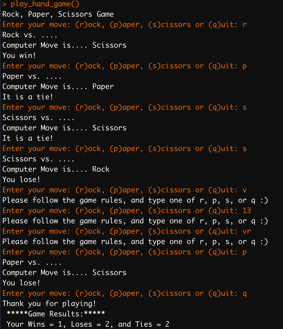
Exercise 6.4 Create a function that allows the user to play a game of rock, paper, scissors against the computer. The function should have the following features:

The user should be prompted to enter their move as a text input (i.e., rock, paper, or scissors).
The computer should randomly select a move.
The program should ensure that the user’s input is a valid move.
After each round, the program should report the result of the game as a text output, either “You win!”, “You lose.”, or “It’s a tie.”
The user should be able to play as many rounds as they wish until they choose to quit.
When the user decides to quit, the program should provide a summary of the number of games won, lost, and tied.

An example of how the function works is provided below.