Chapter 13 Semantic Representations: Word Embeddings
# --- Core Text Analytics Framework (Quanteda) ---
library(quanteda)             # Main framework for managing and analyzing text
library(quanteda.textmodels)   # Statistical models for scaling and classifying text
library(quanteda.textplots)    # Specialized visualizations like word clouds and networks
library(quanteda.textstats)    # Computation of text statistics (frequency, keyness, etc.)

# --- Data Science & Machine Learning Tools ---
library(tidyverse)             # Collection of tools (dplyr, ggplot2, etc.) for data wrangling
library(word2vec)              # Training and utilizing word embedding models
library(Rtsne)                 # T-Distributed Stochastic Neighbor Embedding for visualization
library(ggrepel)               # Prevents overlapping text labels in ggplot2 charts
library(wordcloud)             # Generation of standard and comparison word clouds
We have finally reached the last chapter of our course materials. My goal for this final module is twofold. First, we will build upon the distributional semantic hypothesis by exploring how word embeddings are trained using neural network architectures. Second, we will integrate the corpus-based methods covered throughout the semester into a cohesive case study, demonstrating a comprehensive workflow for quantitative corpus analysis.
13.1 A Typical Data Analysis Workflow
Our Research Questions
- In Mandarin pop songs, what are the general emotional attitudes toward the concepts of “Man” and “Woman”? Are there differences?
- Do these emotional connections vary among different artists?
- Through this simple example, we will guide you through the typical steps, workflow, and details required for a data science research project.
13.2 Data Collection
- The first step in data science is data collection capability.
- Use existing corpora or collect your own.
- Web scraping is usually the first step for beginners.
- We scraped Mandarin pop lyrics and related information (artist, title, lyricist, composer, etc.) from the MOJIM lyrics website.
13.3 Data Preprocessing
Common Text Processing
- Typical text data preprocessing includes:
- Text Normalization
- Text Tokenization
- Text Enrichment/Annotation
- Data often contains noise; the first step is usually Data Wrangling—removing characters unrelated to the research topic to facilitate subsequent analysis.
- In this example, we removed the following characters from the original lyrics:
- Extra whitespace and line breaks
- Punctuation and special symbols
- English characters and Arabic numerals
## --- PURPOSE: A custom cleaning pipeline to remove noise from raw Chinese lyrics ---
preprocess <- function(doc) {

  ## 1. Normalizing Line Breaks:
  ## Collapses multiple consecutive newlines into a single one to maintain structure
  doc <- str_replace_all(doc, "\n+", "\n")

  ## 2. Filtering Non-Linguistic Noise:
  ## Uses Unicode properties to remove:
  ## \p{P} - Punctuation (e.g., !, ?, 。)
  ## \p{S} - Symbols (e.g., ¥, ★, ❤)
  ## \p{N} - Numbers (e.g., 1, 2, 3)
  ## These are replaced with spaces to prevent accidental merging of words
  doc <- str_replace_all(doc, "[\\p{P}\\p{S}\\p{N}]", " ")

  ## 3. Filtering Latin Characters (English):
  ## Specifically removes lowercase (\p{Ll}) and uppercase (\p{Lu}) letters
  ## Useful when you want to focus exclusively on Mandarin Chinese analysis
  doc <- str_replace_all(doc, "[\\p{Ll}\\p{Lu}]", " ")

  ## 4. Normalizing White Space:
  ## Removes both standard spaces and the Chinese full-width space (\u3000)
  doc <- str_replace_all(doc, "[ \u3000]+", "")

  ## 5. Final Formatting & Trimming:
  ## Re-collapses newlines after the cleaning steps above
  doc <- str_replace_all(doc, "\n+", "\n")

  ## Splits document into lines, trims whitespace from ends, and joins back together
  lines <- str_split(doc, "\n")[[1]]
  doc <- paste(str_trim(lines), collapse = "\n")

  return(doc)
}

## --- APPLICATION ---
## Uses purrr::map_chr to apply the 'preprocess' function to every entry in the
## lyric column, returning a clean character vector
lyric <- map_chr(song_sub$lyric, preprocess)[1] "你說的話 在我心中生了根\n愛得很深 所以心會疼\n記憶 在我的心中翻滾\n是不是每一個人 都像我一樣笨\n只怕再問 對彼此都太殘忍\n我能感覺 另外一個人\n我等 等笑容換成淚痕\n愛在崩潰的時候 比較真\n太多疑問 知道答案又如何\n原來容忍不需要天份 只要愛錯一個人\n心痛比快樂更真實 愛為何這樣的諷刺\n我忘了這是第幾次 一見你就無法堅持\n孤獨比擁抱更真實 愛讓人失去了理智\n會不會是我太自私 拒絕更寂寞的日子\n放不開 也看不見未來\n難道這種不完美 才是愛情真實的樣子\n太多疑問 知道答案又如何\n原來容忍不需要天份 只要愛錯一個人\n心痛比快樂更真實 愛為何這樣的諷刺\n我忘了這是第幾次 一見你就無法堅持\n孤獨比擁抱更真實 愛讓人失去了理智\n會不會是我太自私 拒絕更寂寞的日子\n孤獨比擁抱更真實 愛讓人失去了理智\n會不會是我太自私 拒絕更寂寞的日子\n放不開 也看不見未來\n難道這種不完美 才是愛情真實的樣子\n感謝\ntang891228\n修正歌詞"[1] "你說的話在我心中生了根\n愛得很深所以心會疼\n記憶在我的心中翻滾\n是不是每一個人都像我一樣笨\n只怕再問對彼此都太殘忍\n我能感覺另外一個人\n我等等笑容換成淚痕\n愛在崩潰的時候比較真\n太多疑問知道答案又如何\n原來容忍不需要天份只要愛錯一個人\n心痛比快樂更真實愛為何這樣的諷刺\n我忘了這是第幾次一見你就無法堅持\n孤獨比擁抱更真實愛讓人失去了理智\n會不會是我太自私拒絕更寂寞的日子\n放不開也看不見未來\n難道這種不完美才是愛情真實的樣子\n太多疑問知道答案又如何\n原來容忍不需要天份只要愛錯一個人\n心痛比快樂更真實愛為何這樣的諷刺\n我忘了這是第幾次一見你就無法堅持\n孤獨比擁抱更真實愛讓人失去了理智\n會不會是我太自私拒絕更寂寞的日子\n孤獨比擁抱更真實愛讓人失去了理智\n會不會是我太自私拒絕更寂寞的日子\n放不開也看不見未來\n難道這種不完美才是愛情真實的樣子\n感謝\n修正歌詞"Word Segmentation (Chinese Preprocessing)
Since Chinese text does not have explicit word boundaries, the next step after initial cleaning is usually “Word Segmentation.”
In the word-segmented version of the lyrics, we use spaces as delimiters between words.
In this implementation, we used
jiebaRfor word segmentation. For more detail, please check the course material, Chinese Text Processing.
[1] "你說的話在我心中生了根\n愛得很深所以心會疼\n記憶在我的心中翻滾\n是不是每一個人都像我一樣笨\n只怕再問對彼此都太殘忍\n我能感覺另外一個人\n我等等笑容換成淚痕\n愛在崩潰的時候比較真\n太多疑問知道答案又如何\n原來容忍不需要天份只要愛錯一個人\n心痛比快樂更真實愛為何這樣的諷刺\n我忘了這是第幾次一見你就無法堅持\n孤獨比擁抱更真實愛讓人失去了理智\n會不會是我太自私拒絕更寂寞的日子\n放不開也看不見未來\n難道這種不完美才是愛情真實的樣子\n太多疑問知道答案又如何\n原來容忍不需要天份只要愛錯一個人\n心痛比快樂更真實愛為何這樣的諷刺\n我忘了這是第幾次一見你就無法堅持\n孤獨比擁抱更真實愛讓人失去了理智\n會不會是我太自私拒絕更寂寞的日子\n孤獨比擁抱更真實愛讓人失去了理智\n會不會是我太自私拒絕更寂寞的日子\n放不開也看不見未來\n難道這種不完美才是愛情真實的樣子\n感謝\n修正歌詞"[1] "你 說 的 話 在 我 心 中 生 了 根 \n 愛 得 很 深 所以 心 會 疼 \n 記憶 在 我 的 心 中 翻滾 \n 是 不 是 每 一 個 人 都 像 我 一樣 笨 \n 只 怕 再 問 對 彼此 都 太 殘忍 \n 我 能 感覺 另外 一 個 人 \n 我 等等 笑容 換成 淚痕 \n 愛 在 崩潰 的 時候 比較 真 \n 太多 疑問 知道 答案 又 如何 \n 原來 容忍 不 需要 天份 只要 愛錯 一 個 人 \n 心痛 比 快樂 更 真實 愛 為何 這樣 的 諷刺 \n 我 忘 了 這 是 第幾 次 一 見 你 就 無法 堅持 \n 孤獨 比 擁抱 更 真實 愛 讓 人 失去 了 理智 \n 會不會 是 我 太 自私 拒絕 更 寂寞 的 日子 \n 放 不 開 也 看 不 見 未來 \n 難道 這 種 不 完美 才 是 愛情 真實 的 樣子 \n 太多 疑問 知道 答案 又 如何 \n 原來 容忍 不 需要 天份 只要 愛錯 一 個 人 \n 心痛 比 快樂 更 真實 愛 為何 這樣 的 諷刺 \n 我 忘 了 這 是 第幾 次 一 見 你 就 無法 堅持 \n 孤獨 比 擁抱 更 真實 愛 讓 人 失去 了 理智 \n 會不會 是 我 太 自私 拒絕 更 寂寞 的 日子 \n 孤獨 比 擁抱 更 真實 愛 讓 人 失去 了 理智 \n 會不會 是 我 太 自私 拒絕 更 寂寞 的 日子 \n 放 不 開 也 看 不 見 未來 \n 難道 這 種 不 完美 才 是 愛情 真實 的 樣子 \n 感謝 \n 修正 歌詞"13.4 Corpus Data Profile
This current dataset collects lyrics from 17 Mandarin male and female singers as text for analysis, totaling 2409 songs.
The selection of these singers was not strictly logical (perhaps reflecting my age ). For higher research rigor, all male and female singers should ideally be included (or a better heuristics for sampling needs to be provided).
- The distribution of songs collected per artist is as follows:
song_sub %>%
  group_by(artist) %>%
  summarize(N=n()) %>%
  ggplot(aes(reorder(artist, N), N)) +
           geom_bar(stat="identity", aes(fill=N), color="white") +
           geom_text(aes(label = N), nudge_y = 10) +
           theme(axis.text=element_text(angle=90))+
  labs(x="Artist", y = "Number of Songs") +
  scale_fill_distiller(palette = "RdYlBu") +
  coord_flip() +
theme(axis.text.y = element_text(angle=0)) 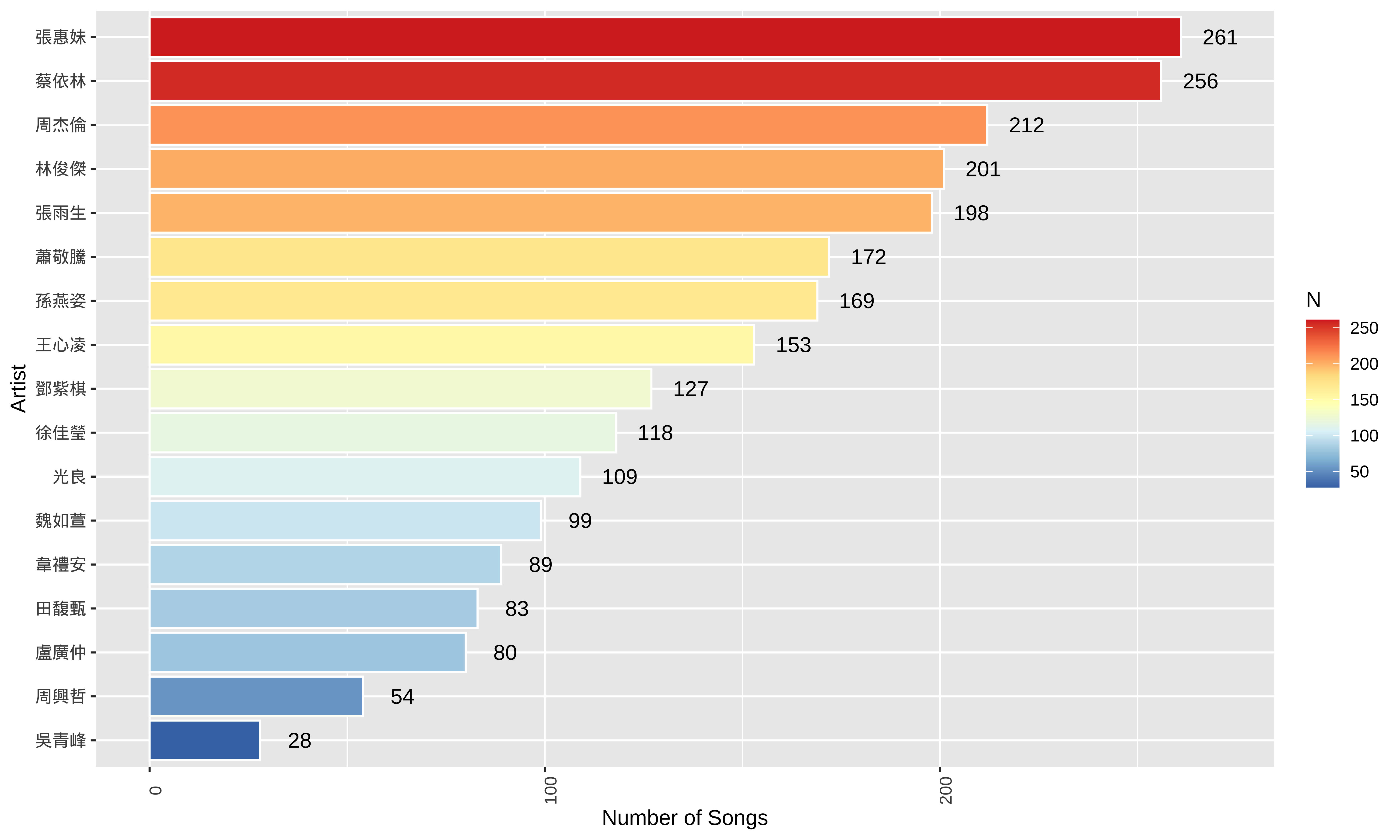
13.5 How do we define the sentiment of “Man” and “Woman” concepts?
To determine which concepts are associated with 男人 (Man) and 女人 (Woman), we can compare two methods:
The Classic Approach: Collocations
Collocations identify words that habitually appear together more frequently than chance. This method focuses on the “company words keep” within a specific text.
- Mechanism: Uses statistical measures to find words that physically appear near the target within a fixed window.
- Intuition: It captures explicit, surface-level associations, such as specific adjectives an artist frequently uses to describe a gender.
- Analysis: We extract these highly linked words and analyze their emotional orientation using sentiment lexicons to see if certain genders are consistently paired with specific moods.
You can utilize the fcm() function introduced in Chapter 12 to extract words co-occurring with MEN and WOMEN within a fixed window size. By calculating the lexical associations of these co-occurrence patterns, you can determine a distinct set of significant collocates for MEN and WOMEN respectively. Ideological interpretations can then be made based on these contrasting collocates.
The Deep Learning Approach: Word Embeddings
Word embeddings map words into a high-dimensional vector space where geometric closeness corresponds to semantic similarity, even if the target words never co-occur in the same sentence. For ideological analysis, this shifting of words into a multi-dimensional space is invaluable because it captures systemic cultural associations and subtle framing biases rather than just explicit declarations.
- Mechanism: The model learns latent relationships based on the Distributional Hypothesis, which states that words occurring in similar contexts share similar meanings.
- Intuition: It captures conceptual neighbors and semantic clusters, revealing deeper, implicit societal associations and latent ideologies that simple keyword frequencies might miss.
- Application for Ideological Analysis: By projecting abstract concepts into a shared vector space, we can mathematically calculate the distance between target categories (such as gender vectors like MEN and WOMEN) and specific evaluative attributes (such as domesticity, career, or emotion clusters). This allows researchers to quantify the systemic, non-obvious biases embedded in a text or an entire corpus, providing empirical evidence of how specific groups or ideas are culturally framed.
Advantages of Word Embeddings
- Continuous Vector Representations: Word embeddings represent words as dense, low-dimensional vectors of real numbers (e.g., 300 dimensions), replacing sparse methods like one-hot encoding. This numerical format allows computers to perform mathematical operations on text.
- The Distributional Hypothesis: The underlying linguistic assumption is that words occurring in similar contexts share similar semantic properties. Embedding algorithms derive meaning by analyzing these co-occurrence patterns across large corpora.
- Representation Learning: These numerical vectors are learned automatically. Through predictive training architectures (like Word2Vec), a network continuously minimizes prediction errors, adjusting coordinates so that distributionally similar words (like cat and dog) are positioned close together in the vector space.
- Foundation for Language Models: These dense vectors serve as the foundational inputs for modern natural language processing, deep learning architectures, and Large Language Models (LLMs), allowing them to capture subtle syntactic and semantic relationships.
Hugging Face operates as a central hub for the open-source artificial intelligence community, hosting thousands of pre-trained embedding models that are publicly accessible for academic and linguistic research. Through the Hugging Face Hub, researchers can download state-of-the-art models for text, speech, and multimodal representations across hundreds of languages. These resources allow you to leverage massive, deeply trained architectures—such as BERT, RoBERTa, and Chinese language models developed by CKIP Lab—without the need for immense local computational power, making advanced representation learning highly accessible for quantitative text analysis.
13.6 A Step-by-Step Training of Word Embeddings
This practical guide walks you through the entire pipeline of training and analyzing predictive word embeddings in R using the word2vec package.
We will move step-by-step from raw token preparation and hyperparameter configuration to model training. Once the embeddings are learned, we can extract semantic neighbors of the seed words (e.g., 男人, 女人) and map the high-dimensional vectors onto a 2D space using t-SNE and PCA.
a. Prepare the Tokens
The word2vec package requires the corpus data to be in the form of a list of word-tokenized character vectors, where each document has been split into independent word units. The most efficient way to prepare your text for this pipeline is to first generate a standard tokens object of your corpus.
## 1. Convert Segmented Text to Tokens:
## Splits the space-separated character strings into individual word units (tokens)
song_sub_tokens <- str_split(song_sub$lyric_wordseg, "\\s+")

## 2. Stopword Preparation:
library(tmcn)
## Retrieve a standard Chinese stopword list and ensure it is in Traditional Chinese
## to match the script used in Mandarin Pop lyrics
stopwords_zh <- toTrad(stopwords("zh", source = "misc"))

## 3. Custom Filtering:
## Add domain-specific noise words commonly found in lyric metadata
stopwords_zh <- c(stopwords_zh, "感謝", "修正", "提供", "歌詞")

## 4. Token Cleaning Pipeline:
song_sub_tokens %>%
  ## Convert the raw list into a quanteda 'tokens' object for efficient processing
  as.tokens() %>%
  ## Remove all functional words and custom noise defined in our stopword list
  tokens_remove(stopwords_zh) %>%
  ## Convert the cleaned tokens back into a standard R list for downstream analysis
  as.list() -> song_sub_tokens
b. Training the Model
To train the embeddings model, we use the word2vec() function.
This function allows you to configure your model by selecting the training architecture—either Skip-gram or CBOW—and adjusting key hyperparameters like vector dimensionality, window size, and iteration count.
## Set a seed to ensure that the stochastic (random) weight initialization
## remains the same every time the code is executed
set.seed(123)

## Model Training Configuration:
model <- word2vec(
  x = song_sub_tokens,         ## Input: A list of character vectors (cleaned tokens)

  ## Architecture: Skip-gram focuses on using a target word to predict context,
  ## which typically handles rare words and semantic nuances better than CBOW
  type = "skip-gram",

  ## Embedding Dimensionality: Maps each word into a 128-dimensional coordinate space
  dim = 128,

  ## Context Window: The model looks at 5 words before and 5 words after the target
  window = 5,

  ## Training Iterations: The algorithm makes 20 complete passes over the dataset
  iter = 20,

  ## Frequency Threshold: Words appearing fewer than 5 times in the corpus are
  ## excluded to ensure the model only learns from sufficient evidence
  min_count = 5,

  ## Parallel Processing: Distributes the computation across 4 CPU cores to reduce training time
  threads = 4
)

## Export the trained model to a binary file so it can be reloaded
## later without re-running the training process
write.word2vec(model, "embeddings/songs_tokens_embeddings.bin")
Within the Word2Vec framework, there are two primary architectures used to learn word embeddings. Both rely on a “sliding window” approach to analyze context, but they differ in their prediction direction.
CBOW (Continuous Bag-of-Words)
- Predicting the target from the context
- Logic: The model takes multiple surrounding “context words” as input and tries to predict the single “target word” in the middle.
- Performance:
- Faster to train than Skip-gram.
- Works well with frequent words.
- Smoothes out distributional information by treating the context as a single “bag” of words.
Skip-gram
- Predicting the context from the target
- Logic: The model takes a single “target word” as input and tries to predict the multiple “context words” that are likely to appear around it.
- Performance:
- Slower to train because it performs more independent predictions.
- Superior at capturing the semantics of rare words and complex relationships.
- Generally preferred for high-quality, large-scale linguistic research.
c. Extracting and Using Embeddings
Once the model is trained, you can convert the word embeddings into a matrix for analysis or perform nearest-neighbor searches.
- Convert to Matrix
This is useful if you want to use the vectors for downstream tasks like clustering or visualization.
## Extract the model into a numeric matrix (Rows = Words, Cols = Dimensions)
embedding_matrix <- as.matrix(model)

## Check dimensions: Returns (Vocabulary Size) x (Vector Size)
dim(embedding_matrix)
[1] 6715 128 [,1] [,2] [,3] [,4] [,5] [,6]
啦啦啦啦啦啦 -0.5565755 0.5403181 -0.1907424 2.2037737 -0.5880290 0.8335724
不行 2.0012131 0.8623514 1.0751743 0.8538892 0.2703077 -1.6228430
灌醉 -0.3714184 0.2764275 -0.8629256 0.1533670 -0.4302930 -0.8786584
遭 -1.0538697 -0.1597221 1.0251306 0.9514959 -0.1472969 -0.4060965
孩子氣 -0.9931604 2.5363295 0.4723191 0.7263509 -0.4221019 1.7803526
[,7] [,8] [,9] [,10]
啦啦啦啦啦啦 -1.1787330 -0.9467657 1.0399548 1.16576743
不行 -0.3668516 -1.6583116 1.1864265 -0.66687912
灌醉 1.3465923 -1.2710948 1.8166435 -0.01753941
遭 0.2323204 -1.3714545 0.0287346 0.71901548
孩子氣 0.2000266 0.8425407 1.5854251 0.70922559d. Finding Semantic Neighbors
To find words that are semantically close to a target word (the most common use case in linguistics):
## Identify the 10 words with the highest cosine similarity to "愛" (Love)
neighbors <- predict(model, newdata = "愛", type = "nearest", top_n = 10)

## Output the result list showing neighbor terms and their similarity scores
print(neighbors)
$愛
term1 term2 similarity rank
1 愛 簡簡單單 0.7016374 1
2 愛 我 0.6994971 2
3 愛 判處 0.6983948 3
4 愛 明白 0.6833066 4
5 愛 你 0.6789176 5
6 愛 不明不白 0.6756501 6
7 愛 真愛 0.6751033 7
8 愛 甩甩 0.6744492 8
9 愛 說 0.6733435 9
10 愛 麥克 0.6722113 10e. Saving and Loading the Model
Since training on large corpora can be time-consuming, you should save your model to a binary file.
f. Visualization
- Principal Component Analysis (PCA):
- It acts as a global linear lens that rotates and projects high-dimensional data to capture the directions of greatest variation. Because it is a deterministic mathematical transformation, it produces the same result every time and excels at preserving the broad, overall structure of the dataset.
- It is particularly useful for identifying clear semantic directions, such as parallel vectors in gender or tense analogies, where the goal is to maintain the relative distances across the entire “map” of word embeddings.
- t-Distributed Stochastic Neighbor Embedding (t-SNE):
- It is a non-linear, probabilistic algorithm designed to prioritize local neighborhoods. It calculates the likelihood that points are neighbors in high-dimensional space and attempts to replicate those specific relationships in a 2D layout.
- While it is stochastic and yields slightly different results depending on the random seed, it is the superior choice for revealing complex, hidden clusters.
- This method is ideal for visualizing how words naturally group into semantic islands that linear methods like PCA might otherwise obscure.
Tsne Demo
## Define a set of focal words for the visualization
target_words <- c('寂寞', '快樂', '難過', '孤單', '高興', '驚訝', '男人', '女人')

## Define a safe extraction function to retrieve neighbors while handling missing vocabulary
get_neighbors <- function(model, target_word, n = 10) {
  ## Convert the model to a matrix for vocabulary checking and vector extraction
  wvs <- as.matrix(model)

  ## Verify if the target word exists in the model to avoid execution errors
  if (!(target_word %in% rownames(wvs))) {
    warning(paste("Word '", target_word, "' not in vocabulary."))
    return(character(0))
  }

  ## Extract the specific embedding vector for the target word
  target_vector <- wvs[target_word, , drop = FALSE]

  ## Identify the nearest neighbors based on the extracted vector
  res <- predict(model, newdata = target_vector, type = "nearest", top_n = n)

  ## Return the character vector of neighboring terms
  return(res[[target_word]]$term)
}

## Build a comprehensive list of words including targets and their top 5 neighbors
all_similar_words <- target_words %>%
  map(~get_neighbors(model, .x, n = 5)) %>%
  unlist() %>%
  union(target_words) %>%
  unique()

## Filter the full embedding matrix to keep only the selected subset of words
wvs <- as.matrix(model)
wvs_subset <- wvs[rownames(wvs) %in% all_similar_words, ]

## Execute t-SNE to compress the 128D vectors into 2D coordinates for plotting
## Perplexity is set low due to the small size of the word subset
set.seed(0)
tsne_out <- Rtsne(wvs_subset, perplexity = 3, max_iter = 10000, check_duplicates = FALSE)

## Prepare a data frame for ggplot2, mapping t-SNE coordinates to X and Y axes
tsne_df <- data.frame(
  X = tsne_out$Y[, 1],
  Y = tsne_out$Y[, 2],
  label = rownames(wvs_subset),
  ## Logical flag to distinguish between original targets and their neighbors
  is_target = rownames(wvs_subset) %in% target_words
)

## Render the 2D map using colors to highlight target concepts versus neighbors
ggplot(tsne_df, aes(X, Y, label = label)) +
  geom_point(aes(color = is_target)) +
  ## Use repel to automatically position labels and prevent overlapping text
  geom_text_repel(aes(color = is_target)) +
  scale_color_manual(values = c("royalblue", "firebrick"),
                     labels = c("Neighbor", "Target Word"),
                     name = "Word Type") +
  theme_minimal() +
  labs(title = "t-SNE Visualization of Word Embeddings")
Guidelines for Determining Perplexity
There is no single “correct” mathematical formula for perplexity, but you can use several heuristics and diagnostics to find the optimal setting.
1. The Sample Size Rule of Thumb
The standard convention in machine learning is to set perplexity between 5 and 50. More importantly, perplexity should scale with the size of your dataset (\(N\)):
- The Bound: Perplexity must always be less than the total number of data points (\(N\)).
- The Ratio: A common safe zone is to set perplexity to roughly 1% to 10% of your dataset size, depending on how dense your clusters are.
How to Evaluate the Sweep Results
When you experiment with different perplexity values, evaluate the plots based on these structural behaviors:
| If you see… | Interpretation | Action |
|---|---|---|
| Points scattered evenly like stars with no clear groupings. | Perplexity is too high for your sample size. | Decrease the perplexity. |
| Every single data point forms its own tiny, isolated cluster of 1 or 2 points. | Perplexity is too low; the model is over-interpreting random noise as local clusters. | Increase the perplexity. |
| Stable, distinct shapes that persist across 2 or 3 consecutive perplexity steps. | The Sweet Spot. These structures are robust and reflect true properties of the high-dimensional space. | Use this value for your final analysis. |
PCA Demo
## Perform PCA to reduce high-dimensional word vectors into two linear components
## center = TRUE shifts the variables to be zero-centered for accurate rotation
pca_out <- prcomp(wvs_subset, center = TRUE, scale. = FALSE)

## Calculate the percentage of variance captured by each principal component
## This helps students understand how much information is retained in the 2D plot
var_explained <- round(100 * pca_out$sdev^2 / sum(pca_out$sdev^2), 1)

## Prepare the plotting data frame using the first two principal components (PC1 and PC2)
pca_df <- data.frame(
  PC1 = pca_out$x[, 1],
  PC2 = pca_out$x[, 2],
  label = rownames(wvs_subset),
  ## Tag target words vs neighbors for visual differentiation
  is_target = rownames(wvs_subset) %in% target_words
)

## Render the PCA map with informative axis labels showing variance explained
ggplot(pca_df, aes(PC1, PC2, label = label)) +
  geom_point(aes(color = is_target), size = 2) +
  ## box.padding ensures enough clear space around labels for readability
  geom_text_repel(aes(color = is_target),
                  box.padding = 0.5) +
  scale_color_manual(values = c("royalblue", "firebrick"),
                     labels = c("Neighbor", "Target Word"),
                     name = "Word Type") +
  theme_minimal() +
  labs(
    title = "PCA Visualization of Word Embeddings",
    subtitle = "Dimensionality reduction using Principal Component Analysis",
    x = paste0("PC1 (", var_explained[1], "%)"),
    y = paste0("PC2 (", var_explained[2], "%)")
  ) +
  theme(legend.position = "bottom")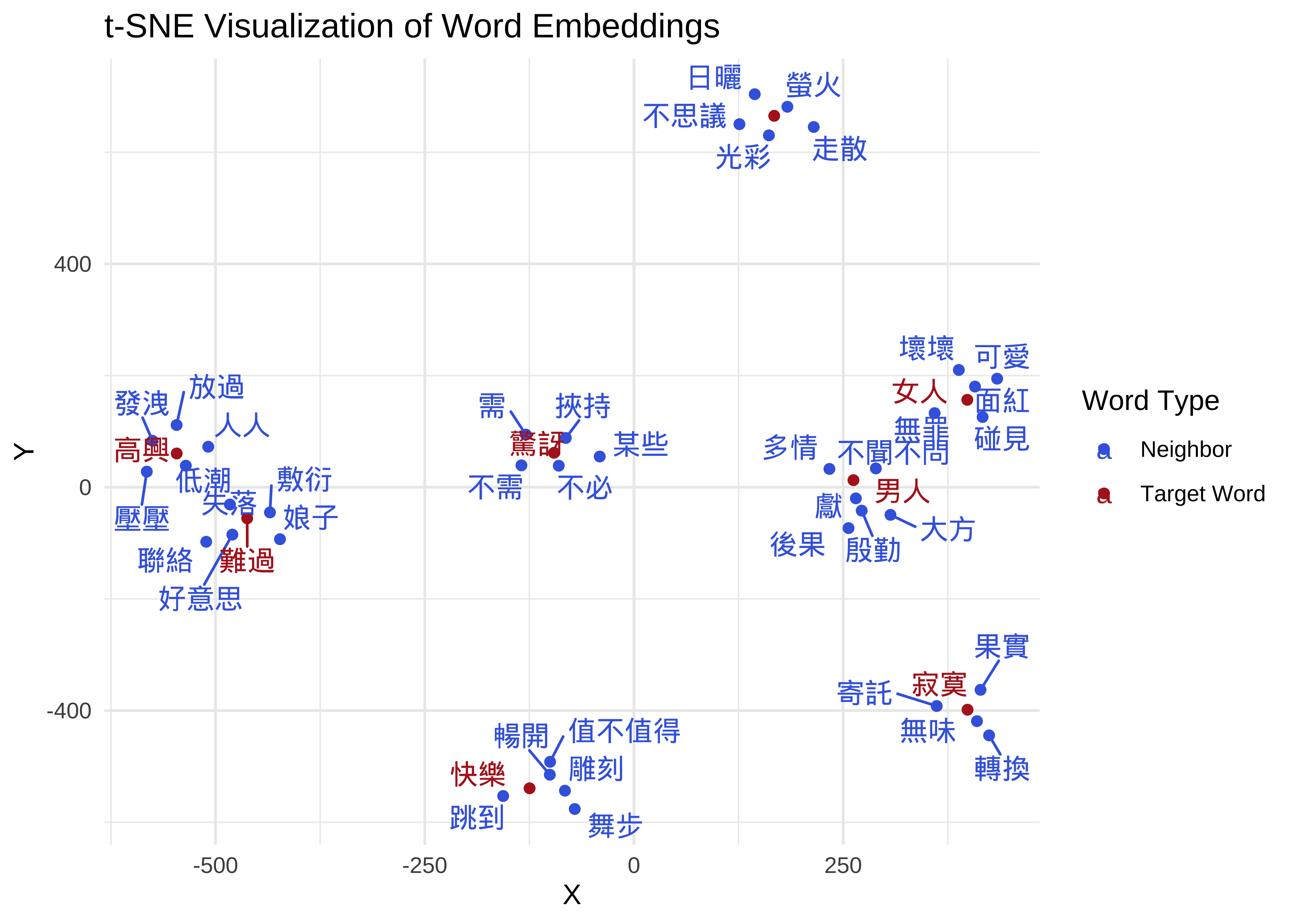
g. Key word2vec Hyperparameters to Consider
| Parameter | Recommended Value | Description |
|---|---|---|
dim |
50 – 300 | Higher dimensions capture more nuance but require more data. |
window |
5 – 10 | Smaller windows capture functional similarity (synonyms); larger windows capture topical similarity. |
type |
“skip-gram” | Skip-gram usually performs better on smaller datasets or rare words. |
iter |
10 – 50 | More iterations can lead to better convergence but take longer. |
13.7 Intuitions for Word Embeddings (Self-Study)
Word embeddings transform words into dense vectors of real numbers, typically across hundreds of dimensions. These numerical mappings are established based on the Distributional Hypothesis, which suggests that words appearing in similar linguistic contexts share similar meanings. By representing linguistic units mathematically, we can move beyond simple string matching to analyze the underlying conceptual space of a corpus.
Semantic Calculation and Lexical Distance
The utility of embeddings stems from the ability to quantify lexical distance. In a high-dimensional vector space, the proximity between two word vectors serves as a proxy for their semantic relationship.
- Cosine Similarity: This is the standard metric for measuring semantic proximity. It calculates the cosine of the angle between two vectors, where a value approaching 1 indicates high similarity and a narrow angle in the vector space.
- Vector Arithmetic: Because these representations are algebraic, they can capture complex relational analogies. This is famously illustrated by the equation:
\[\text{Vector}(\text{"King"}) - \text{Vector}(\text{"Man"}) + \text{Vector}(\text{"Woman"}) \approx \text{Vector}(\text{"Queen"})\]
A Quick Example based on Sinca Corpus
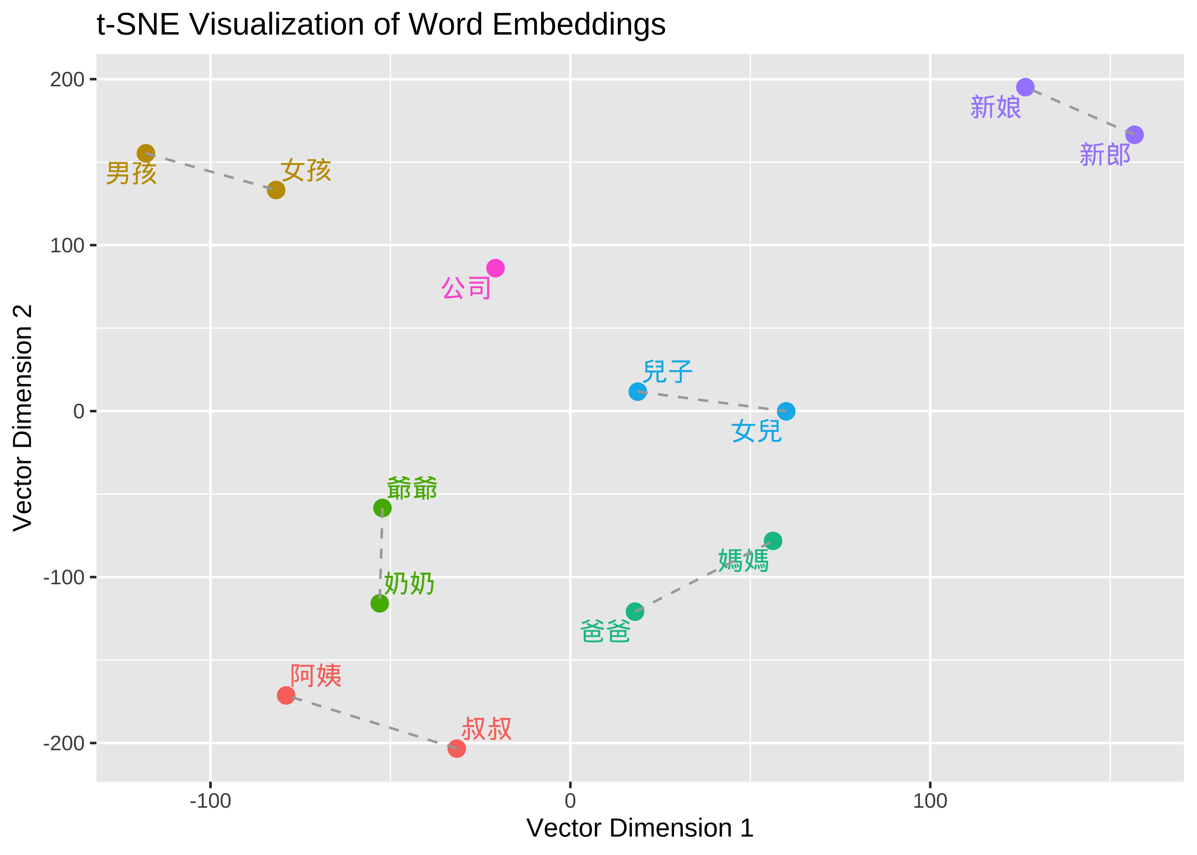
The following R code utilizes a pre-trained embeddings model, sinica_model, to demonstrate how embeddings organize relational concepts. By visualizing these vectors, we can observe how the model mathematically encodes social and familial structures.
a. Dimensionality Reduction (t-SNE)
To make 300-dimensional data interpretable for human vision, we apply t-SNE. This algorithm compresses high-dimensional data into a 2D plane while prioritizing the preservation of local neighborhoods, ensuring that closely related words remains clustered together.
b. Capturing Parallelism
In the visualization, dashed lines connect pairs such as 叔叔 (Uncle) — 阿姨 (Aunt) and 爸爸 (Dad) — 媽媽 (Mom). When these lines appear roughly parallel and of similar length, it provides visual evidence that the model has identified a consistent “gender” dimension. The mathematical “shift” required to move from a male term to its female counterpart is nearly identical across different kinship pairs.
c. Clustering by Semantic Domain
Words within the same semantic field naturally gravitate toward the same region of the vector space. For instance, kinship terms like 爺爺 (Grandpa) and 奶奶 (Grandma) will be significantly closer to each other than to unrelated entities like 公司 (Company), reflecting their frequent co-occurrence in similar textual environments.
We apply this embedding methodology to identify words semantically similar to 男人 and 女人 within the lyrics database. This allows for a deeper downstream analysis of the specific sentiment or emotional traits associated with these gendered concepts across different artists.
13.8 Embeddings Training
13.8.1 Train a base word embedding model on the entire dataset
Previously, we trained a global embedding model (songs_tokens_embeddings.bin) based on the entire song lyrics corpus for illustration.
The next step is to train artist-specific embedding models. By generating distinct models for each individual artist, we can identify and compare the specific sets of lexical items that are conceptually closest to the target concepts, 男人 and 女人, within that particular artist’s body of work.
## Load the pre-trained Word2Vec model into the R environment
base_embeddings <- read.word2vec("embeddings/songs_tokens_embeddings.bin")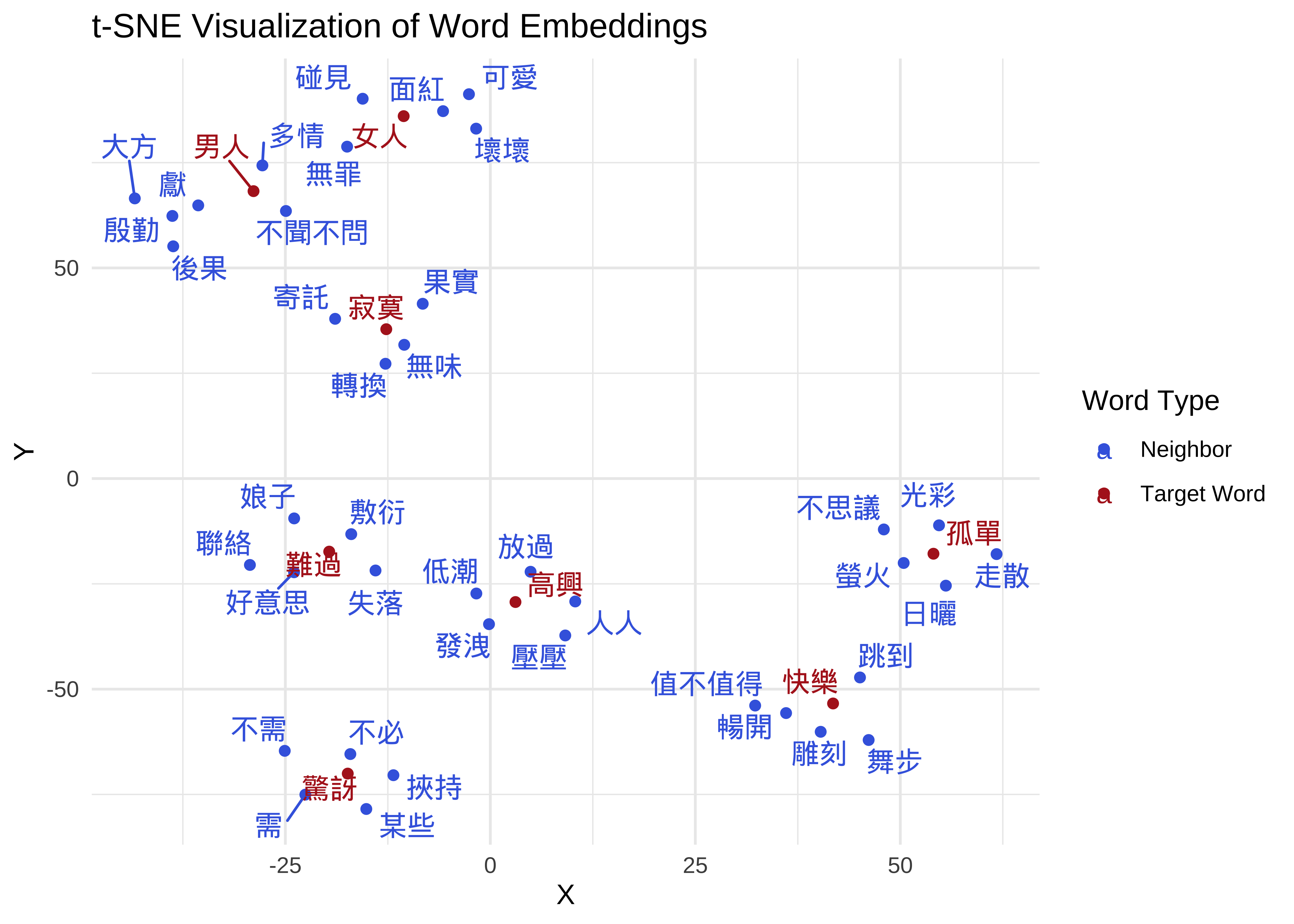
13.8.2 Artist-Specific Model Training
- For each artist, we train an artist-specific word embedding model.
- We split the entire database into 17 sub-corpora based on artists. We then trained an independent “Artist Word Embedding” model for each artist.
## Identify all unique artist names in the dataset to drive the loop
all_artists <- unique(song_sub$artist)

## Iteratively train a separate semantic model for every artist found
for (artist in all_artists) {

  ## Subset the tokenized lyrics belonging specifically to the current artist
  sub_lyric <- song_sub_tokens[song_sub$artist == artist]

  ## Print a progress message to the console showing current artist and song count
  message(sprintf("Working on %s with %d songs", artist, length(sub_lyric)))

  ## Train an artist-specific embedding model
  ## This captures the unique word associations and poetic style of the individual
  model_art <- word2vec(
    x = sub_lyric,      ## Input: Current artist's token list
    type = "skip-gram", ## Architecture: Better for small, specific datasets
    dim = 128,          ## Vector size: Kept consistent with the base model
    window = 5,         ## Context window size
    min_count = 5,      ## Minimum frequency threshold for a word to be included
    iter = 20,          ## Training epochs
    threads = 4         ## Parallel processing cores
  )

  ## Save the resulting model as a binary file named after the artist
  write.word2vec(model_art, sprintf("embeddings/%s.bin", artist))
}
13.8.3 Identify nearest neighbors
- From each artist-specific word embedding model, we found the 100 words most similar to “Man” and “Woman” respectively for subsequent sentiment analysis.
- Each artist generated 200 words semantically similar to “Man” and “Woman” (100 each), totaling \(17 \times 200 = 3400\) words.
Out-of-Vocabulary Issue
- When training individual embedding models for each artist to analyze concepts like 男人 (Man) and 女人 (Woman), the primary challenge is the Out-of-Vocabulary (OOV) problem. This occurs when a model cannot process a word because it was not present—or not frequent enough—in the specific training data for that artist.
## Define global parameters for the analysis
search_terms <- c("男人", "女人")
top_n_neighbors <- 100
model_dir <- "embeddings"
output_path <- "data/artist_semantic_neighbors.csv"

## Load the global Base Model to provide a semantic reference for all artists
base_model_path <- file.path(model_dir, "base_embeddings.bin")
if (!file.exists(base_model_path)) {
  stop("Base model not found!")
}
base_model <- read.word2vec(base_model_path)
## Extract the embedding matrix for fast vocabulary lookups and vector projection
base_wvs <- as.matrix(base_model)

## Identify all artist-specific binary model files in the directory
## Excludes the main base embedding file from the processing list
model_files <- list.files(model_dir, pattern = "\\.bin$", full.names = TRUE)
model_files <- model_files[!str_detect(model_files, "embeddings\\.bin")]

## Function to extract semantic neighbors while handling Out-of-Vocabulary (OOV) terms
extract_artist_data <- function(model_path, terms, local_base_matrix) {
  artist_name <- str_replace(basename(model_path), "\\.bin$", "")
  message(paste("Processing artist:", artist_name))

  ## Load the individual artist's trained embedding space
  model_art <- read.word2vec(model_path)
  wvs_art <- as.matrix(model_art)

  ## Iterate through the target concepts to extract their local semantic context
  map_df(terms, function(term) {
    ## Check if the artist has used the term enough times to have a native vector
    if (term %in% rownames(wvs_art)) {
      target_vector <- wvs_art[term, , drop = FALSE]
      mode_type <- "direct"
    } else {
      ## FALLBACK: If word is missing, project the vector from the global Base Model
      ## This allows us to see what an artist "would" associate with a word they rarely use
      message(sprintf("  -> '%s' OOV for %s. Using Base Model projection.", term, artist_name))

      if (term %in% rownames(local_base_matrix)) {
        target_vector <- local_base_matrix[term, , drop = FALSE]
        mode_type <- "base_projection"
      } else {
        return(NULL)
      }
    }

    ## Extract top neighbors within the artist's specific semantic landscape
    res <- predict(model_art, newdata = target_vector, type = "nearest", top_n = top_n_neighbors)

    if (is.null(res[[1]])) return(NULL)

    ## Return results in a tidy format for comparative analysis
    data.frame(
      artist = artist_name,
      target_concept = term,
      extraction_mode = mode_type,
      neighbor_word = res[[1]]$term,
      similarity = res[[1]]$similarity,
      stringsAsFactors = FALSE
    )
  })
}

## Execute the extraction across all found artist models
all_simwords <- map_df(model_files, ~extract_artist_data(.x, search_terms, base_wvs))

## Export the consolidated data to a CSV for visualization and sentiment analysis
write.csv(all_simwords, output_path, row.names = FALSE)
message("Done! Results saved to data/artist_semantic_neighbors.csv")

## Display the final data frame
all_simwords[1] 3128 5If we analyze 17 artists with 100 neighbors for each of the two target concepts (男人 and 女人), the resulting data frame would theoretically contain 3,400 rows. However, our current all_simwords data frame contains only 3128 rows. Take a moment to inspect the data on your own to see if you can determine why these rows are missing.
13.9 Sentiment Analysis
Analyzing the Sentiment Distribution of Neighboring Words
- What proportion of the words conceptually close to 男人 (men) carry a positive/negative connotation? Furthermore, how many of these neighboring words express happiness, sadness, or anger?
- What proportion of the words conceptually close to 女人 (women) carry a positive/negative connotation? Furthermore, how many of these neighboring words express happiness, sadness, or anger?
Check the Dictionary! Sentiment Dictionary!
- Sentiment analysis ranges from simple valence models that categorize feelings as positive or negative to more granular discrete models, such as Ekman’s, which identify specific emotional states like joy, anger, or sadness.
- Currently, there are a few publicly available Chinese sentiment dictionaries. In this small study, we used the NRC Emotion Dictionary.
- NRC is primarily an English sentiment dictionary, but the authors used automatic translation to expand it to over 100 languages worldwide.
- We used the Chinese version provided by NRC (Please note the translation accuracy).
- See: Saif Mohammad and Peter Turney (2013). Crowdsourcing a Word-Emotion Association Lexicon. Computational Intelligence, 29 (3), 436-465, 2013.
The National Taiwan University Sentiment Dictionary (NTUSD) is an established, widely used linguistic resource developed for Chinese natural language processing and opinion mining. Curated by the Natural Language Processing Laboratory at NTU, it contains over 11,000 entries explicitly categorized into distinct lists of positive and negative words. Because it was specifically optimized for Traditional Chinese text structures and cultural idioms, it serves as an excellent baseline lexicon for researchers analyzing valence, stance, and sentiment trends in Taiwanese digital media, literature, and social discourse.
## Load the NRC Emotion Lexicon and standardize the column name for Chinese words
nrc_dict <- read_tsv("demo_data/NRC-Emotion-Lexicon/OneFilePerLanguage/Chinese-Traditional-NRC-EmoLex.txt") %>%
  rename(Chinese = `Chinese-Traditional Word`)

## Preview the raw dictionary structure
head(nrc_dict)
## Create an emotion-focused dataset (Anger, Anticipation, Disgust, Fear, Joy, Sadness, Surprise, Trust)
nrc_emotion <- nrc_dict %>%
## Select specific emotion categories and the word column
select(anger:joy, sadness:trust, Chinese) %>%
## Transform from wide to long format (each word-emotion pair becomes a row)
pivot_longer(anger:trust, names_to = "emotion") %>%
rename(word = Chinese) %>%
## Keep only entries where the word is actually associated with the emotion (score >= 1)
filter(value >= 1)
head(nrc_emotion)## Create a sentiment-focused dataset (Positive vs. Negative)
nrc_sentiment <- nrc_dict %>%
## Select the binary sentiment columns
select(positive:negative, Chinese) %>%
## Transform to long format for easier joining with text data
pivot_longer(positive:negative, names_to = "sentiment") %>%
rename(word = Chinese) %>%
## Filter for active sentiment associations
filter(value >= 1)
head(nrc_sentiment)Distribution of NRC Sentiment Lexicon
nrc_sentiment %>%
  count(sentiment) %>%
  ggplot(aes(reorder(sentiment,-n), n, fill=n)) +
  geom_bar(stat="identity", color="white") +
  scale_fill_distiller(palette = "RdYlBu")+
  labs(x = "Sentiment Types in NRC",
       y = "Number of Words",
       title = "Distributions of Words Across Different Emotions in NRC")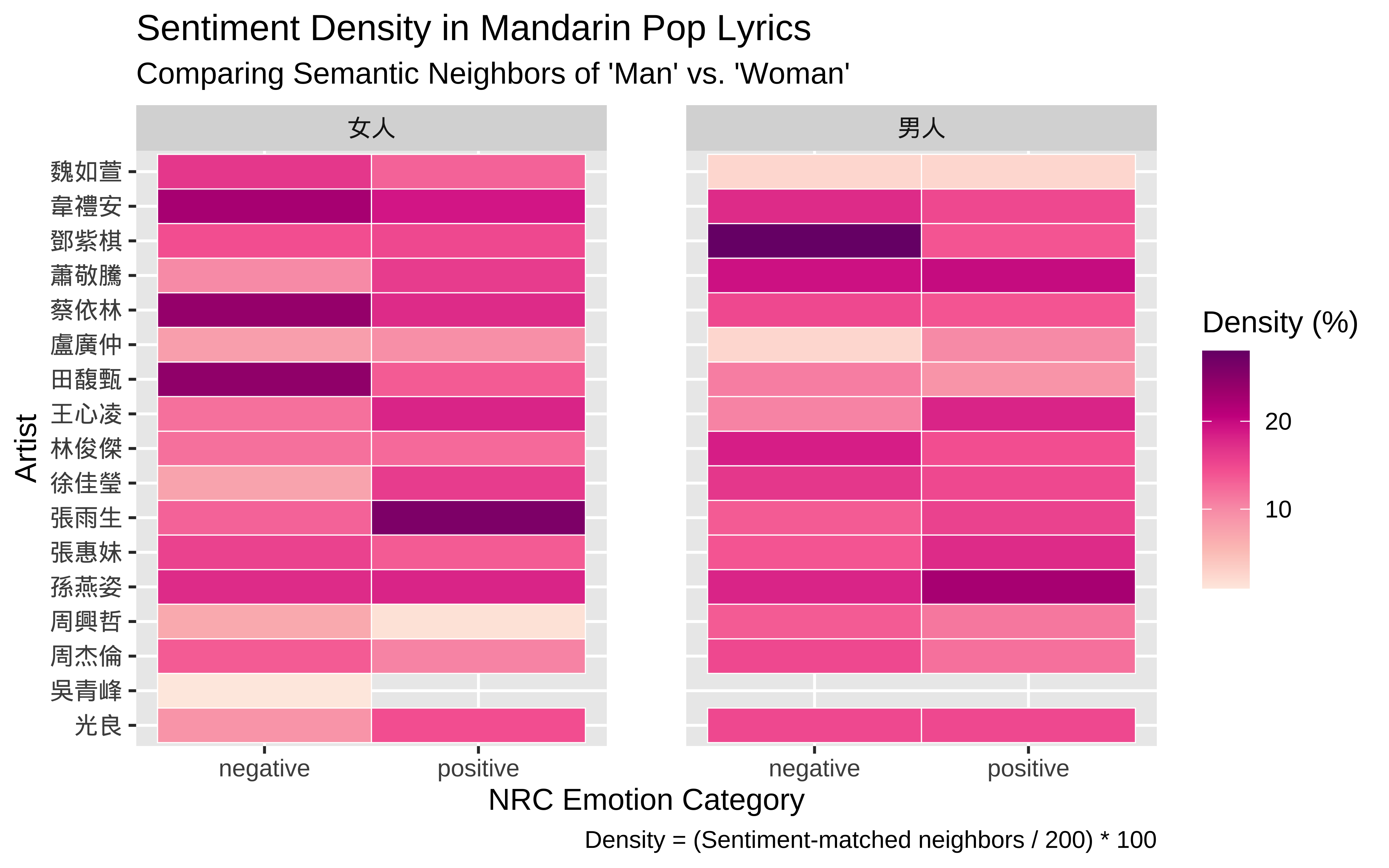
Distribution of NRC Emotion Lexicon
nrc_emotion %>%
  count(emotion) %>%
  ggplot(aes(reorder(emotion,-n), n, fill=n)) +
  geom_bar(stat="identity", color="white") +
  scale_fill_distiller(palette = "RdYlBu")+
  labs(x = "Emotion Types in NRC",
       y = "Number of Words",
       title = "Distributions of Words Across Different Emotions in NRC")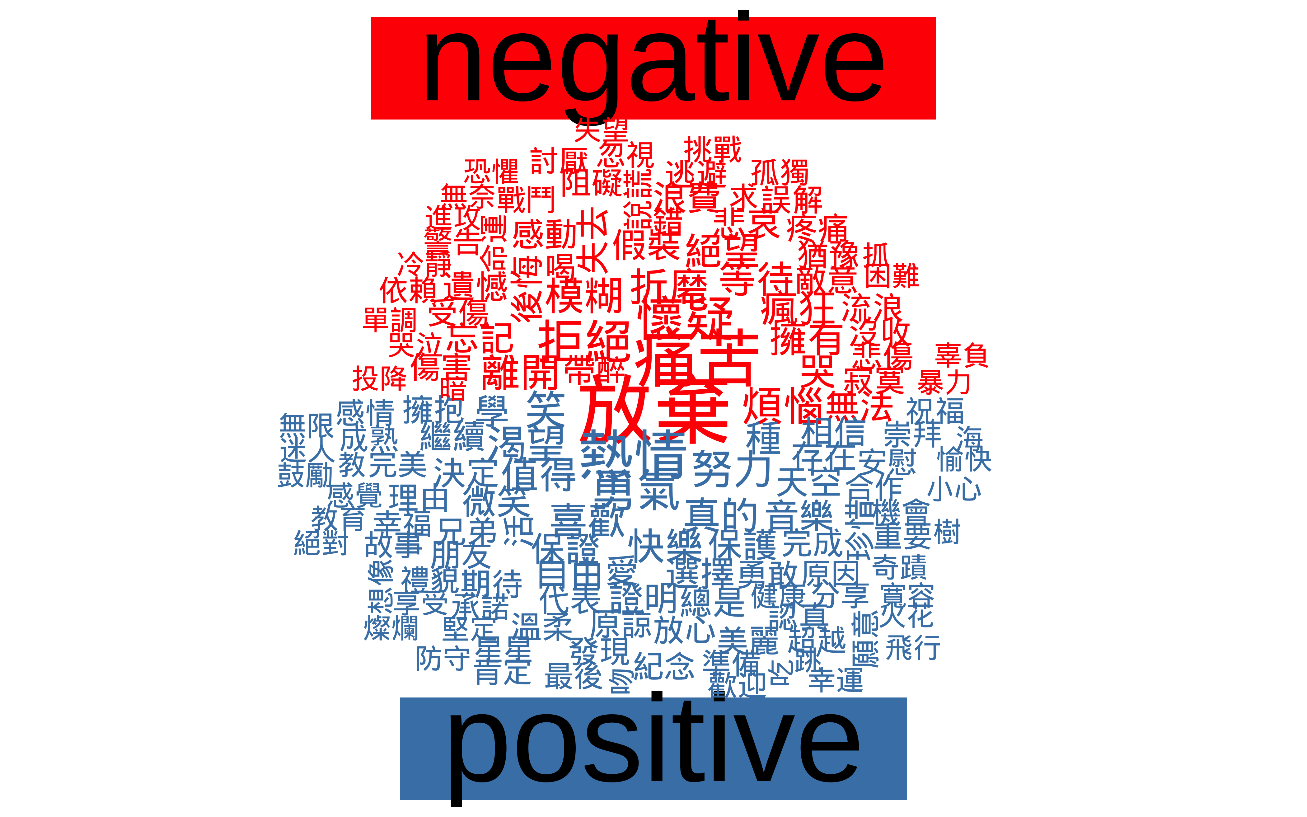
13.10 Mapping 男人/女人 Neighbors to NRC Sentiment Dictionary
We map each neighbor word to its corresponding sentiment label from the NRC dictionary.
## Perform an inner join to match neighboring words with their sentiment labels
## many-to-many handles words that may carry multiple sentiment tags
sentiment_results <- all_simwords %>%
  inner_join(nrc_sentiment, by = c("neighbor_word" = "word"), relationship= "many-to-many") %>%
  distinct(artist, target_concept, neighbor_word, sentiment)

head(sentiment_results)
We then calculate a simple sentiment density score: for each artist, for each target word (男人 vs. 女人), the percentage of positive/negative words among the neighbors.
sentiment_summary<- sentiment_results %>%
  # 1. Group by both the artist and the specific target word
  group_by(artist, target_concept) %>%

  # 2. Calculate density scores based on categorical labels
  summarise(
    neighbor_type = n_distinct(neighbor_word),
    pos_count = sum(sentiment == "positive", na.rm = TRUE),
    neg_count = sum(sentiment == "negative", na.rm = TRUE),

    # Density score is the proportion of affective words relative to total neighbors (N)
    pos_density = pos_count / neighbor_type,
    neg_density = neg_count / neighbor_type,
    .groups = "drop"
  )


head(sentiment_summary)
sentiment_summary_long <- sentiment_summary %>%
select(artist, target_concept, neg_density, pos_density) %>%
pivot_longer(cols = c(pos_density, neg_density),
names_to = "sentiment",
values_to = "density") %>%
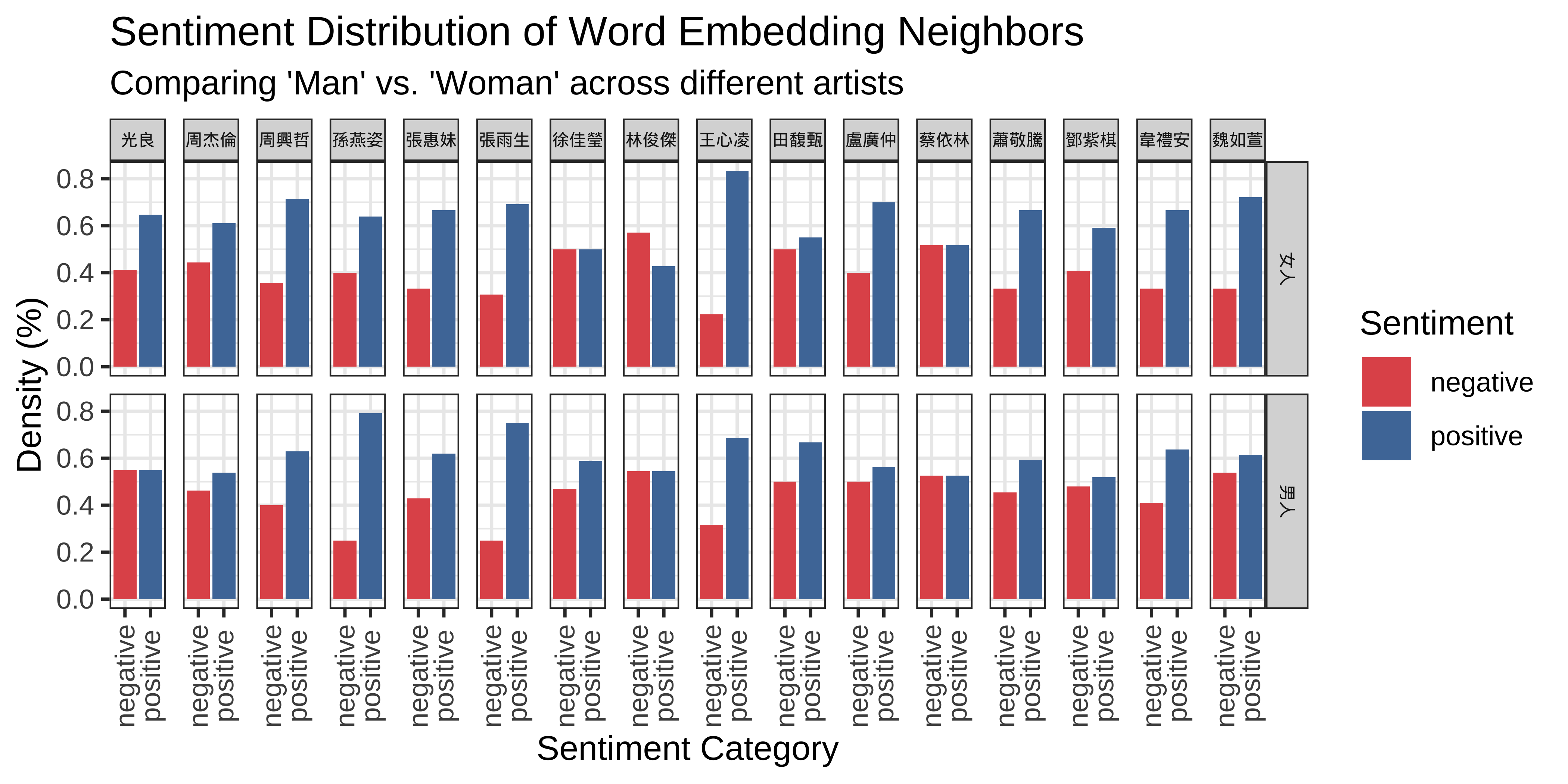
mutate(sentiment = fct_recode(sentiment, "positive" = "pos_density", "negative" = "neg_density"))Visualization of Results: Sentiment
## Render a barplot
ggplot(sentiment_summary_long, aes(x = sentiment, y = density, fill = sentiment)) +
  # Create the bars
  geom_bar(stat = "identity") +
  # Split the plot into two panels based on the target_concept
  #facet_wrap(~target_concept, ncol=1) +
  facet_grid(target_concept ~ artist) +
  scale_fill_manual(values = c("positive" = "#4E79A7", "negative" = "#E15759")) +
  theme_bw() +
  theme(axis.text.x = element_text(angle = 90, vjust = 0.5),
        strip.text = element_text(size = rel(0.5), face = "bold")) +
  labs(
    title = "Sentiment Distribution of Word Embedding Neighbors",
    subtitle = "Comparing 'Man' vs. 'Woman' across different artists",
    x = "Sentiment Category",
    y = "Density (%)",
    fill = "Sentiment"
) 
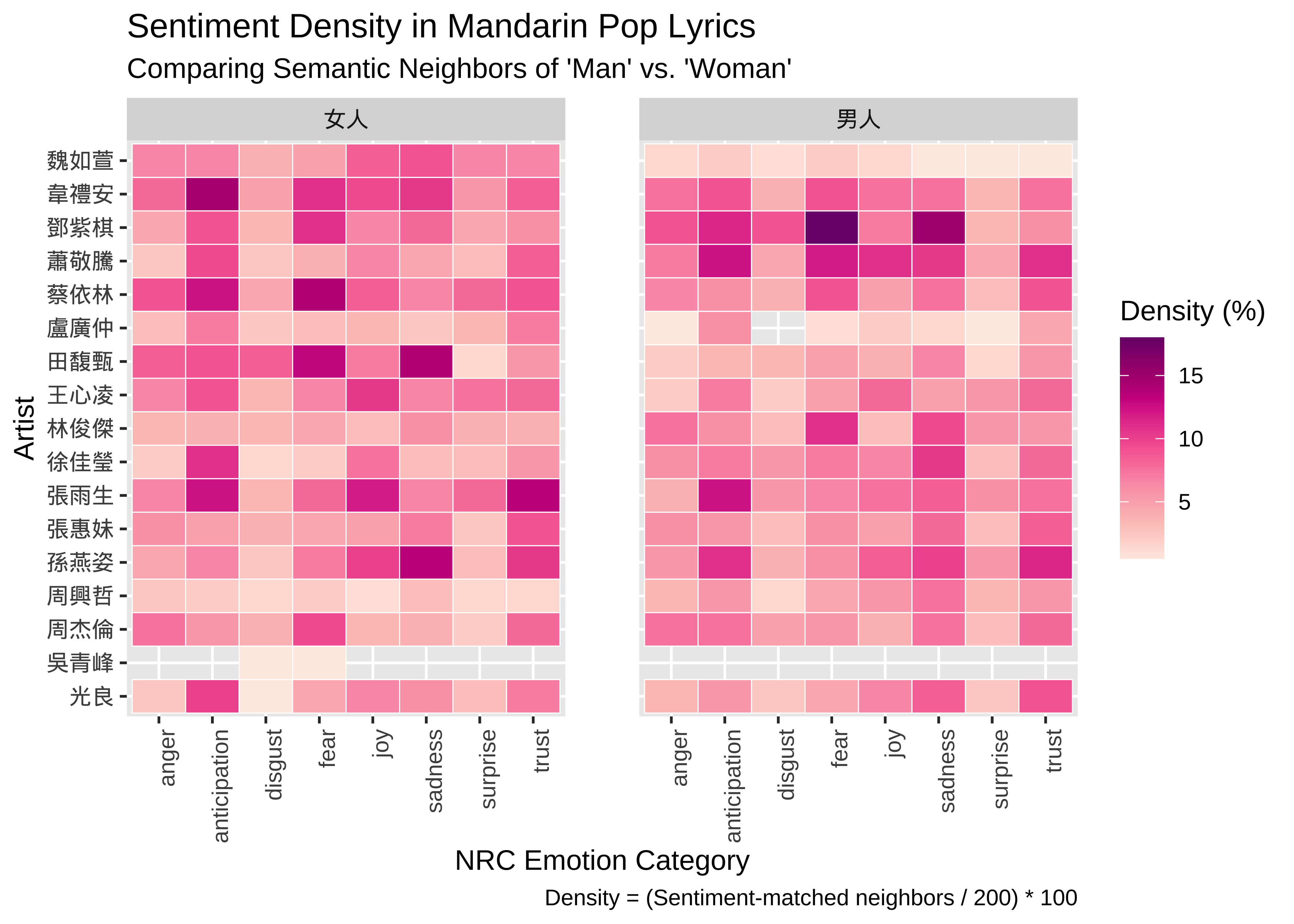
## Render a heatmap to identify broad emotional patterns and artist clusters
ggplot(sentiment_summary_long, aes(x = sentiment, y = artist, fill = density)) +
  ## Use white borders between tiles to improve visual clarity
  geom_tile(color = "white", size = 0.2) +
  ## Separate the visualization into "Man" and "Woman" panels
  facet_wrap(~target_concept) +
  ## Apply a Red-Purple gradient to highlight areas of high sentiment density
  scale_fill_distiller(palette = "RdPu", direction = 1, name = "Density (%)") +
  labs(
    title = "Sentiment Density in Mandarin Pop Lyrics",
    subtitle = "Comparing Semantic Neighbors of 'Man' vs. 'Woman'",
    x = "NRC Emotion Category",
    y = "Artist",
    caption = "Density = (Sentiment-matched neighbors / All Neighbors) * 100"
  ) +
  ## Increase spacing between the faceted panels for better legibility
  theme(
    panel.spacing = unit(2, "lines")
  )
Post-hoc Analysis: Exploring 男人 Sentiment-relevant Neighbors
## MALE
sentiment_results %>%
  count(sentiment, neighbor_word, target_concept, sort = TRUE) %>%
  filter(target_concept == "男人") %>%
  select(-target_concept) %>%
  # Reshape data from long to wide format
  pivot_wider(names_from = sentiment, values_from = n, values_fill = 0) %>%
  # comparison.cloud requires a matrix with row names
  column_to_rownames("neighbor_word") %>%
  comparison.cloud(colors = c("red", "steelblue"),
                   max.words = 150,
                   scale = c(2.5, 0.8),
                   random.order = F,
                   title.size = 4,
                   title.bg.colors = c("red", "steelblue"))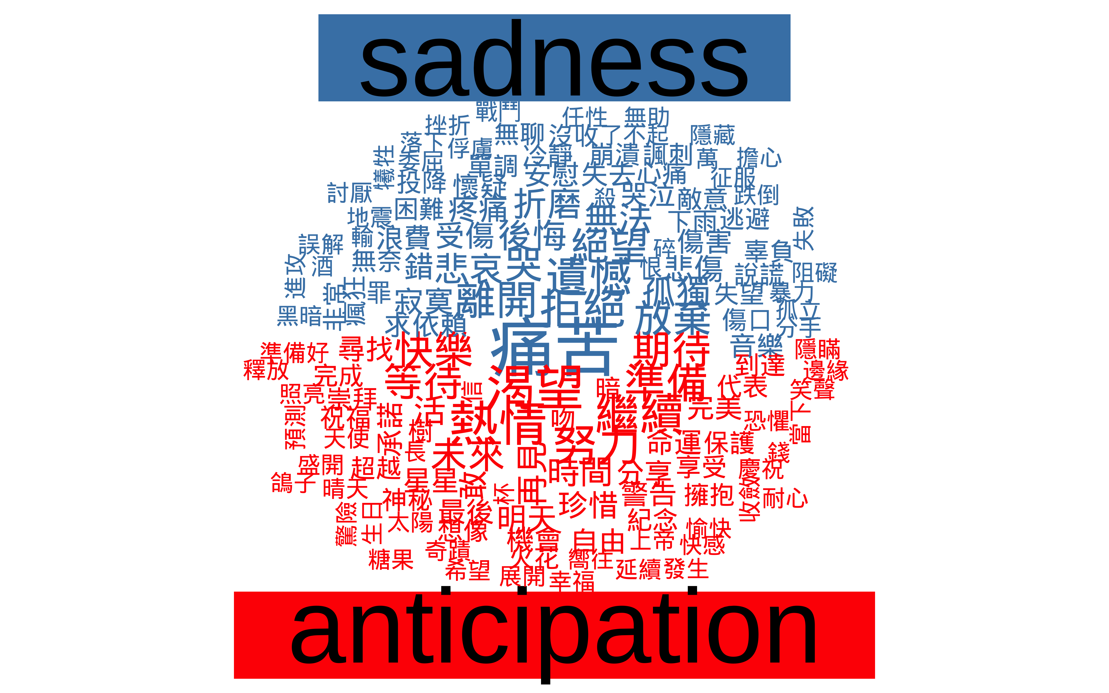
Post-hoc Analysis: Exploring Sentiment-relevant 女人 Neighbors
## FEMALE
sentiment_results %>%
  count(sentiment, neighbor_word, target_concept, sort = TRUE) %>%
  filter(target_concept == "女人") %>%
  select(-target_concept) %>%
  # Reshape data from long to wide format
  pivot_wider(names_from = sentiment, values_from = n, values_fill = 0) %>%
  # comparison.cloud requires a matrix with row names
  column_to_rownames("neighbor_word") %>%
  comparison.cloud(colors = c("red", "steelblue"),
                   max.words = 150,
                   scale = c(2.4, 0.6),
                  random.order = F,
                   title.size = 4,
                   title.bg.colors = c("red", "steelblue"))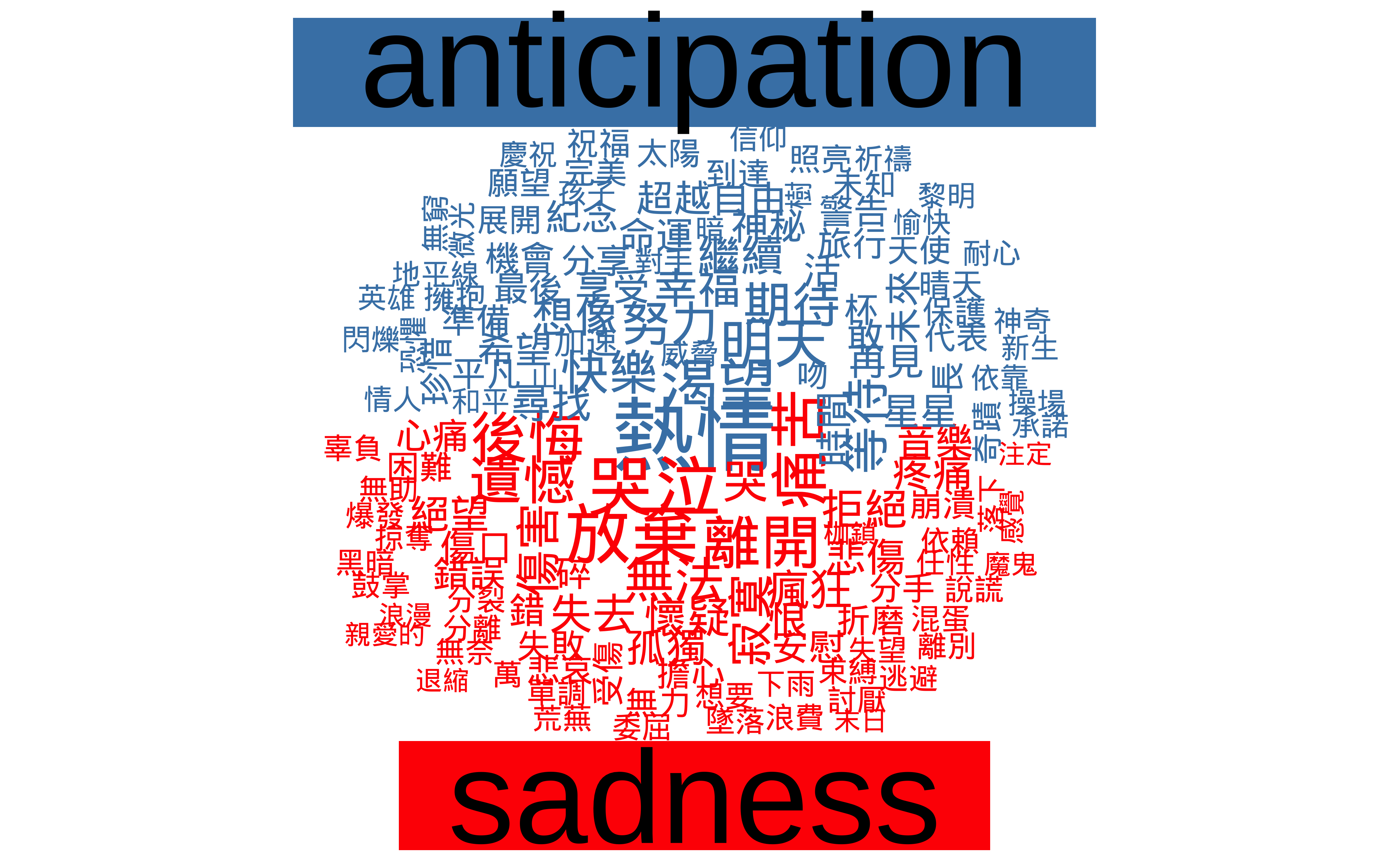
Simple Statistical Analysis (Positive/Negative Binary Sentiment)
# --- Step 1: Fit Two-Way ANOVA with Interaction ---
# Evaluates main effects (target_concept, sentiment) and their interaction (*)
anova_model <- aov(density ~ target_concept * sentiment, data = sentiment_summary_long)

# --- Step 2: Display Significance Table ---
summary(anova_model)
Df Sum Sq Mean Sq F value Pr(>F)
target_concept 1 0.0022 0.0022 0.257 0.614
sentiment 1 0.6614 0.6614 78.158 1.83e-12 ***
target_concept:sentiment 1 0.0169 0.0169 1.994 0.163
Residuals 60 0.5077 0.0085
---
Signif. codes: 0 '***' 0.001 '**' 0.01 '*' 0.05 '.' 0.1 ' ' 1# --- Step 3: Diagnostic Visualization ---
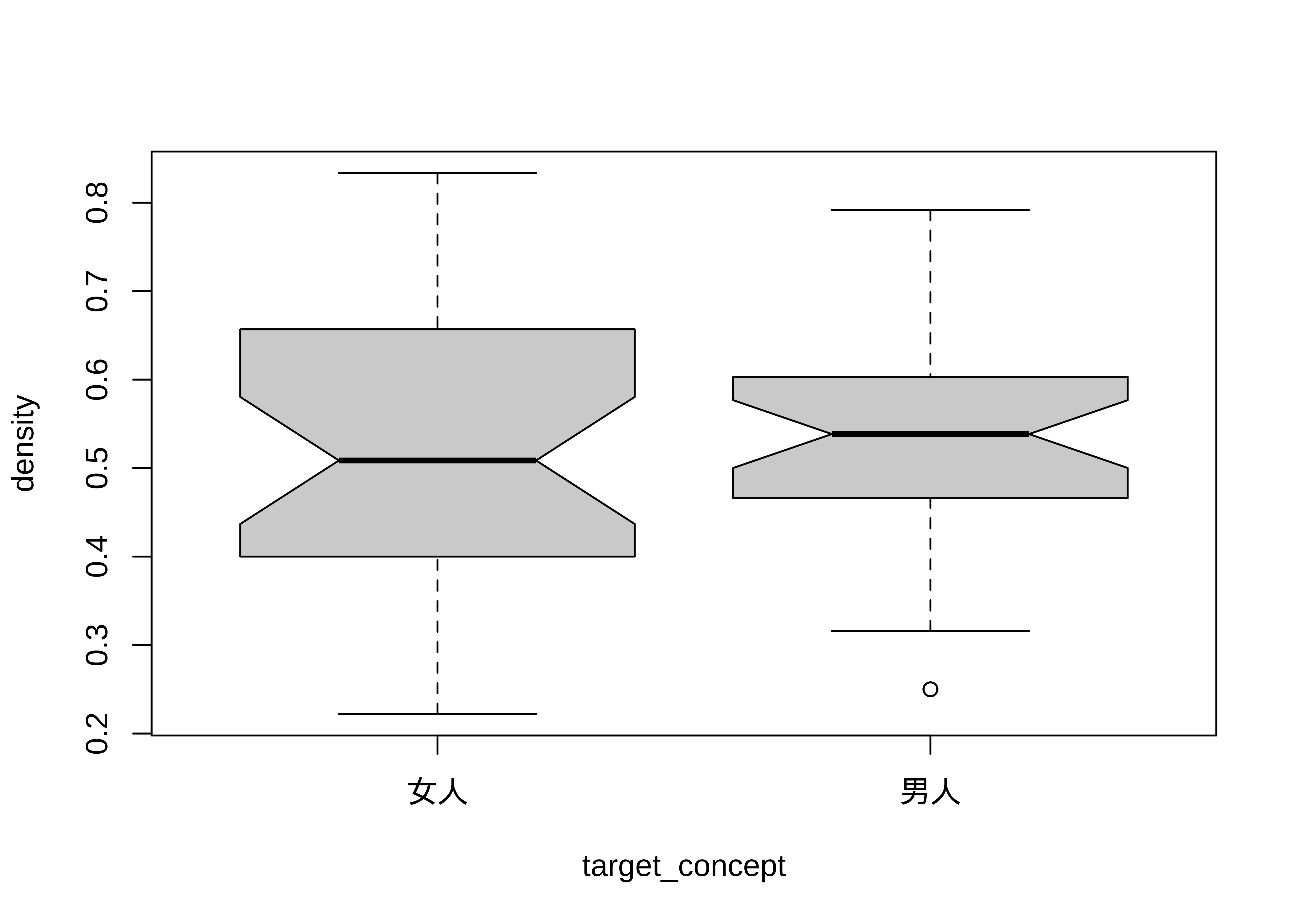
# Generates notched boxplots to compare density distributions across sentiment types
boxplot(density ~ sentiment, notch = TRUE, data = sentiment_summary_long)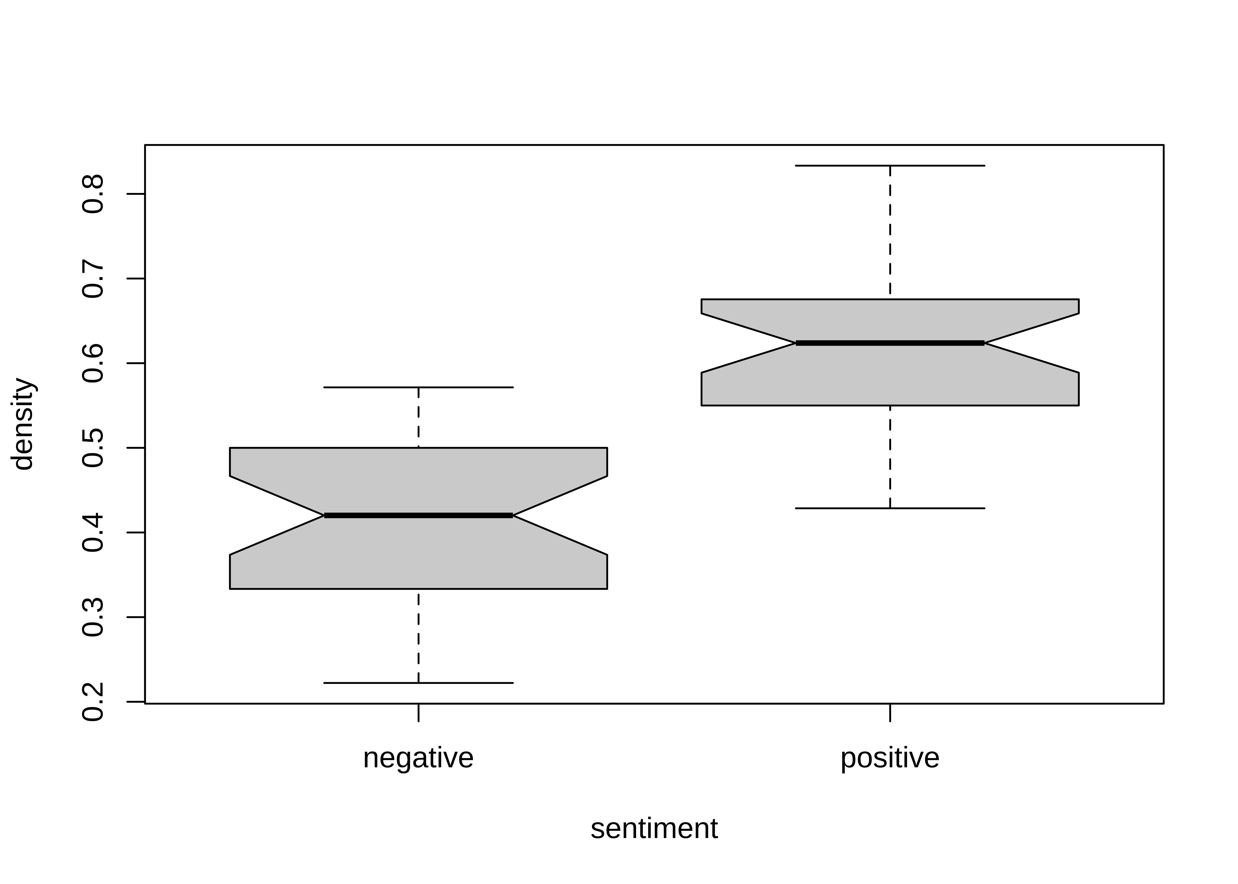
# --- Generate Interaction Plot Directly from Raw Long Data ---
ggplot(sentiment_summary_long, aes(x = target_concept, y = density, color = sentiment, group = sentiment)) +
  # 1. Calculate and plot the mean points
  stat_summary(fun = mean, geom = "point", size = 3.5) +

  # 2. Calculate and draw the connecting interaction lines between those means
  stat_summary(fun = mean, geom = "line", size = 1.2) +

  # 3. Optional but recommended: Add 95% Confidence Interval error bars
  # This shows the statistical variation among the 17 artists for each point
  stat_summary(fun.data = mean_cl_normal, geom = "errorbar", width = 0.1, alpha = 0.6) +

  # Formatting and Styling
  scale_y_continuous(labels = scales::percent) +
  scale_color_manual(values = c("positive" = "#238b45", "negative" = "#cb181d")) +
  theme_minimal(base_family = "Arial") +
  labs(
    title = "Sentiment x Target Concept Interaction Plot",
    subtitle = "Density means with 95% CI error bars",
    x = "Target Concept",
    y = "Sentiment Density",
    color = "Sentiment Profile"
  ) +
  theme(
    plot.title = element_text(face = "bold", size = 13),
    legend.position = "top"
  )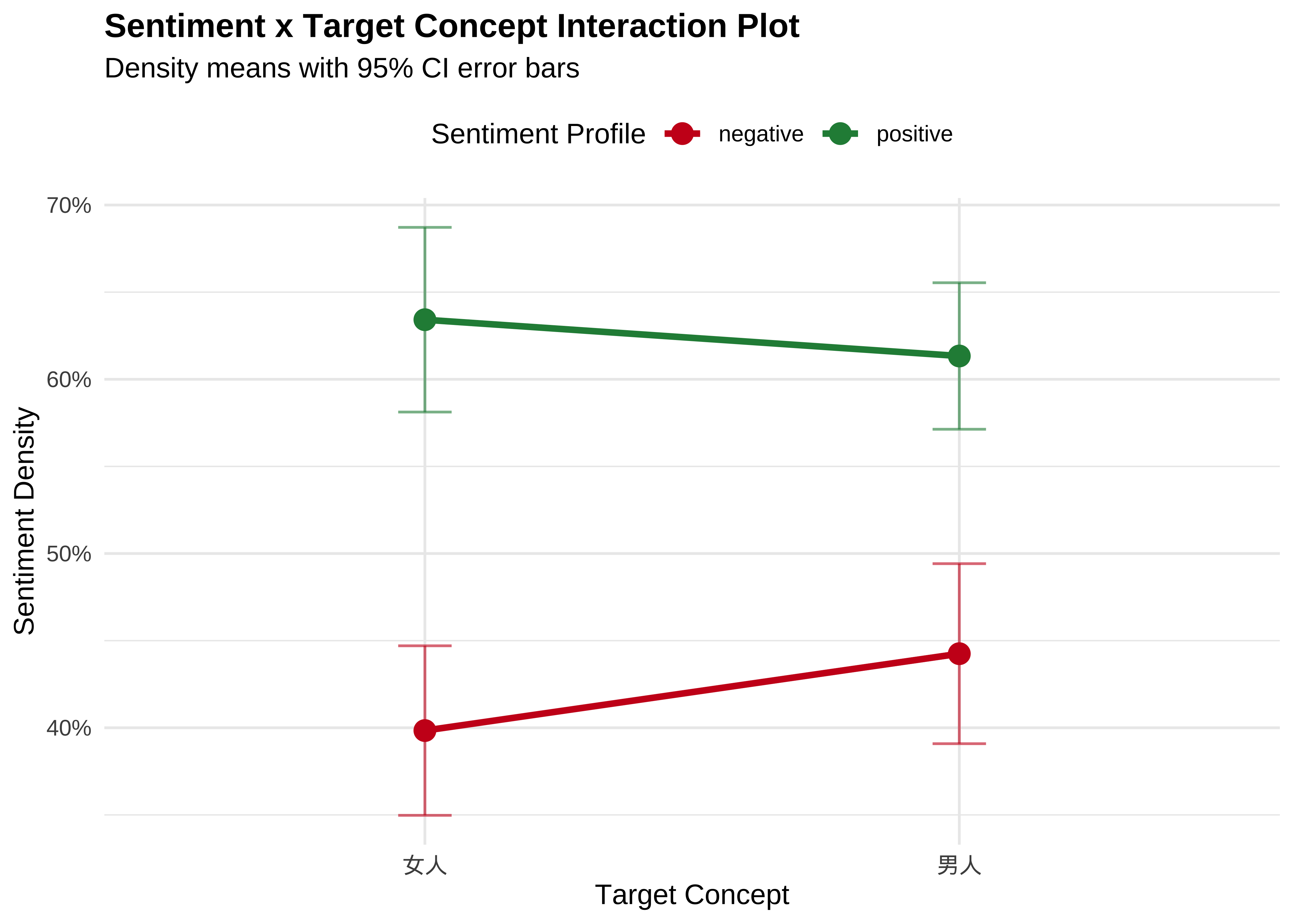
With only 17 artists, our current sample size is relatively small. There are several clear paths to refine and expand this analysis—such as increasing the artist sample, implementing more advanced statistical frameworks, or incorporating additional textual metadata. I will leave these avenues open for you to explore further depending on your research interests.
13.11 Conclusion
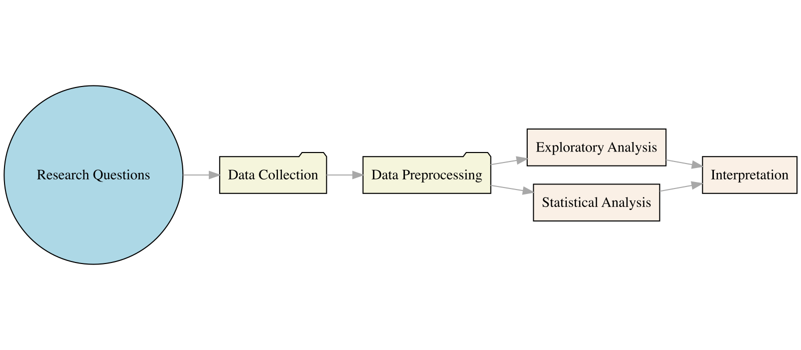
Corpus Analysis and Computer Science
- Research Questions & Hypothesis
- Data Collection (Corpus, Web-Crawling, Other Text Digitizations)
- Data Preprocessing (Text Pre-processing, Data Wrangling)
- Data Analysis (Exploratory Data Analysis & Statistics)
- Interpretation (Data Visualization, Reproducible Reports)