Chapter 4 Corpus Analysis: A Start

In this chapter, I will demonstrate how to perform a basic corpus analysis after you have collected data. I will show you some of the most common ways that people work with the text data.

4.1 Installing quanteda

There are many packages that are made for computational text analytics in R. You may consult the CRAN Task View: Natural Language Processing for a lot more alternatives.

To start with, this tutorial will use a powerful package, quanteda, for managing and analyzing textual data in R. You may refer to the official documentation of the package for more detail.

quanteda is not included in the default R installation. Please install the package if you haven’t done so.

install.packages("quanteda")
install.packages("readtext")

Also, as noted on the quanteda documentation, because this library compiles some C++ and Fortran source code, you will need to have installed the appropriate compilers.

  • If you are using a Windows platform, this means you will need also to install the Rtools software available from CRAN.
  • If you are using macOS, you should install the macOS tools.

If you run into any installation errors, please go to the official documentation page for additional assistance.

library(tidyverse)
library(quanteda)
library(readtext)
library(tidytext)

packageVersion("quanteda")
[1] '3.2.4'

4.2 Building a corpus from character vector

To demonstrate a typical corpus analytic example with texts, I will be using a pre-loaded corpus that comes with the quanteda package, data_corpus_inaugural. This is a corpus of US presidential inaugural address texts, and metadata for the corpus from 1789 to present.

data_corpus_inaugural
Corpus consisting of 59 documents and 4 docvars.
1789-Washington :
"Fellow-Citizens of the Senate and of the House of Representa..."

1793-Washington :
"Fellow citizens, I am again called upon by the voice of my c..."

1797-Adams :
"When it was first perceived, in early times, that no middle ..."

1801-Jefferson :
"Friends and Fellow Citizens: Called upon to undertake the du..."

1805-Jefferson :
"Proceeding, fellow citizens, to that qualification which the..."

1809-Madison :
"Unwilling to depart from examples of the most revered author..."

[ reached max_ndoc ... 53 more documents ]
class(data_corpus_inaugural)
[1] "corpus"    "character"

We create a corpus() object with the pre-loaded corpus in quantedadata_corpus_inaugural:

corp_us <- corpus(data_corpus_inaugural) # save the `corpus` to a short obj name

After the corpus is loaded, we can use summary() to get the metadata of each text in the corpus, including word types and tokens as well. This allows us to have a quick look at the size of the addressess made by all presidents.

summary(corp_us)

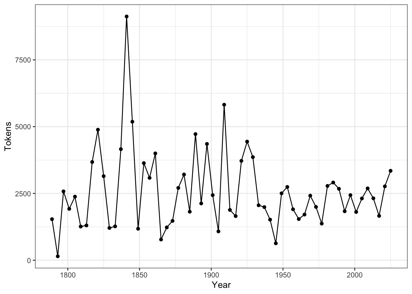
If you like to add document-level metadata information to each document in the corpus object, you can use docvars(). These document-level metadata information is referred to as docvars (document variables) in quanteda.

docvars(corp_us, "country") <- "US"

The advantages of these docvars is that we can easily subset the corpus based on these document-level variables (i.e., a new corpus can be extracted/created based on logical conditions applied to docvars):

corpus_subset(corp_us, Year > 2000) %>%
  summary
require(ggplot2)

corp_us %>%
  summary %>%
  ggplot(aes(x = Year, y = Tokens, group = 1)) +
    geom_line() +
    geom_point() +
    theme_bw()


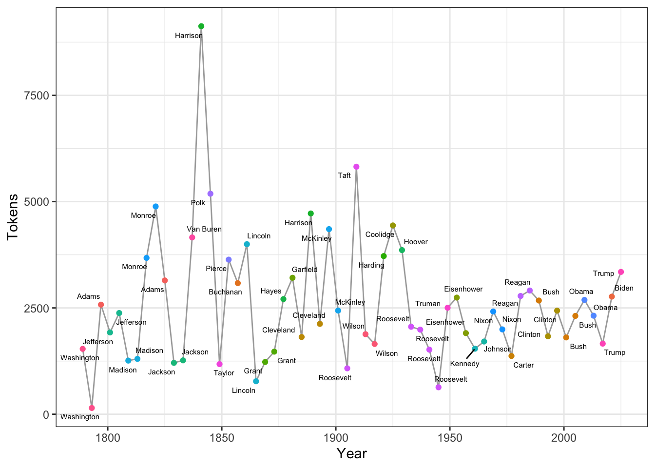
Exercise 4.1 Could you reproduce the above line plot and add information of President to the plot as labels of the dots?

Hints: Please check ggplot2::geom_text() or more advanced one, ggrepel::geom_text_repel()

So the idea is that as long as you can load the text data into a character vector, you can easily create an corpus object with quanteda::corpus().

The library readtext provides a very effective function readtext() for you to load text data from external files. Please check its documentation for more effective usages.

For example, if you have downloaded the file gutenberg.zip and stored it in demo_data, you can load in the gutenberg corpus as follows:

gutenberg <- readtext(file = "demo_data/gutenberg.zip")
gutenberg_corp <- corpus(gutenberg)
summary(gutenberg_corp)

4.3 Keyword-in-Context (KWIC)

Keyword-in-Context (KWIC), or concordances, are the most frequently used method in corpus linguistics. The idea is very intuitive: we get to know more about the semantics of a word by examining how it is being used in a wider context.

We first tokenize the corpus using tokens() and then we can use kwic() to perform a search for a word and retrieve its concordances from the corpus:

## word tokenization
corp_us_tokens <- tokens(corp_us)
## concordances
kwic(corp_us_tokens, "terror")

kwic() returns a data frame, which can be easily exported to a CSV file for later use.

Please note that kwic(), when taking a corpus object as the argument, will automatically tokenize the corpus data and do the keyword-in-context search on a word basis. Yet, the recommended way is to tokenize the corpus object first with tokens() before you perform the concordance analysis with kwic().

The pattern you look for cannot be a linguistic pattern across several words. We will talk about how to extract phrasal patterns/constructions later. Also, for languages without explicit word boundaries (e.g., Chinese), this may be a problem with quanteda. We will talk more about this in the later chapter on Chinese Texts Analytics.

4.4 KWIC with Regular Expressions

For more complex searches, we can use regular expressions as well in kwic(). For example, if you want to include terror and all its other related word forms, such as terrorist, terrorism, terrors, you can create a regular expression for the concordances.

kwic(corp_us_tokens, "terror.*", valuetype = "regex") %>%
  data.frame

By default, the kwic() is word-based. If you like to look up a multiword combination, use phrase():

kwic(corp_us_tokens, phrase("our country")) %>%
  data.frame

It should be noted that the output of kwic includes not only the concordances (i.e., preceding/subsequent co-texts + the keyword), but also the sources of the texts for each concordance line. This would be extremely convenient if you need to refer back to the original discourse context of the concordance line.

After a series of trial and error attempts, it seems that phrase() also supports regular expression search. If we want to extract the concordances of a multiword pattern defined by a regular expression, we can specify the regular expression on a word basis and change the valuetype to be regex.

It is less clear to me how we can use the regular expression to retrieve multiword patterns of variable sizes with kwic().

kwic(corp_us_tokens, 
     phrase("^(the|our)$ ^countr.+?$"), 
     valuetype = "regex") %>%
  data.frame
kwic(corp_us_tokens, 
     phrase("^(be|was|were)$ ^(\\w+ly)$ ^(\\w+ed)$"), 
     valuetype = "regex") %>%
  data.frame

Exercise 4.2 Please create a bar plot, showing the number of uses of the word country in each president’s address. Please include different variants of the word, e.g., countries, Countries, Country, in your kwic() search.


4.5 Tidy Text Format of the Corpus

So far our corpus is a corpus object defined in quanteda. In most of the R standard packages, people normally follow the using tidy data principles to make handling data easier and more effective.

As described by Hadley Wickham (Wickham & Grolemund, 2017), tidy data has a specific structure:

  • Each variable is a column
  • Each observation is a row
  • Each type of observational unit is a table

Essentially, it is an idea of making an abstract object (i.e., corpus) a more intuitive data structure, i.e., a data.frame, which is easier for human readers to work with.

With text data like a corpus, we can also define the tidy text format as being a data.frame with one-token-per-row.

  • A token can be any meaningful unit of the text, such as a word that we are interested in using for analysis, and tokenization is the process of splitting text into tokens.
  • In computational text analytics, the token (i.e., each row in the data frame) is most often a single word, but can also be an n-gram, a sentence, or a paragraph.

The tidytext package in R is made for the handling of the tidy text format of the corpus data. With a tidy data format of the corpus, we can manipulate the text data with a standard set of tidy tools and packages, including dplyr, tidyr, and ggplot2.

The tidytext package includes a function, tidy(), to convert the corpus object from quanteda into a document/text-based data.frame.

library(tidytext)
corp_us_tidy <- tidy(corp_us) # convert `corpus` to `data.frame`
class(corp_us_tidy)
[1] "tbl_df"     "tbl"        "data.frame"

4.6 Processing Flowchart

Figure 4.1: Computational Text Processing Flowchart

4.7 Frequency Lists

4.7.1 Word (Unigram)

To get a frequency list of words, word tokenization is an important step for corpus analysis because words are a meaningful linguistic unit in language. Also, word frequency lists are often indicative of many important messages (e.g., the semantics of the documents).

The tidytext provides a powerful function, unnest_tokens() to tokenize a data frame with larger linguistic units (e.g., texts) into one with smaller units (e.g., words). That is, the unnest_tokens() convert a text-based data frame (each row is a text document) into a token-based data frame(each row is a token splitted from the text).

corp_us_words <- corp_us_tidy %>%
  unnest_tokens(output = word, # new base unit column name
                input = text,  # original base unit column name
                token = "words") # tokenization method

corp_us_words

The unnest_tokens() is optimized for English tokenization of smaller linguistic units, such as words, ngrams, sentences, lines, and paragraphs (check ?unnest_tokens()).

To handle Chinese data, however, we need to be more careful. We probably need to define own ways of tokenization method in unnest_tokens(…, token = …).

We will discuss the principles for Chinese text processing in a later chapter.

Please note that by default, token = “words” would normalize the texts to lower-casing letters. Also, all the non-word tokens are automatically removed. If you would like to preserve the casing differences and the punctuations, you can include the following arguments in unnest_tokens(…, token = “words”, strip_punct = F, strip_numeric = F).

Now we can count the word frequencies by making use of the dplyr library:

corp_us_words_freq <- corp_us_words %>%
  count(word, sort = TRUE)


corp_us_words_freq

4.7.2 Bigrams

Frequency lists can be generated for bigrams or any other multiword combinations as well. The key is we need to convert the text-based data frame into a bigram-based data frame.

corp_us_bigrams <- corp_us_tidy %>%
  unnest_tokens(
    output = bigram, # new base unit column name
    input = text, # original base unit column name
    token = "ngrams", # tokenization method
    n = 2
  )

corp_us_bigrams

To create bigram frequency list:

corp_us_bigrams_freq <- corp_us_bigrams %>% 
  count(bigram, sort=TRUE)
corp_us_bigrams_freq
sum(corp_us_words_freq$n) # size of unigrams
[1] 137939
sum(corp_us_bigrams_freq$n) # size of bigrams
[1] 137880

Could you explain the difference between the total numbers of unigrams and bigrams?

Exercise 4.3 Based on the bigram-based data frame, how can we create a frequency list showing each president’s uses of bigrams with the first-person plural pronoun we as the first word.

In the output, please present the most frequently used bigram in each presential addresss only. If there are ties, present all of them.

Arrange the frequency list according to the year, the president’s last name, and the token frequency of the bigram.

Exercise 4.4 The function unnest_tokens() does a lot of work behind the scene. Please take a closer look at the outputs of unnest_tokens() and examine how it takes care of the case normalization and punctuations within the sentence. Will these treatments affect the frequency lists we get in any important way? Please elaborate.

4.7.3 Ngrams (Lexical Bundles)

corp_us_trigrams <-  corp_us_tidy %>%
  unnest_tokens(trigrams, text, token = "ngrams", n = 3)

corp_us_trigrams

We then can examine which n-grams were most often used by each President:

corp_us_trigrams %>%
  count(President, trigrams) %>%
  group_by(President) %>%
  top_n(3, n) %>%
  arrange(President, desc(n))

Exercise 4.5 Please subset the top 3 trigrams of President Don. Trump, Bill Clinton, John Adams, from corp_us_trigram.


4.7.4 Frequency and Dispersion

When looking at frequency lists, there is another distributional metric we need to consider: dispersion.

An n-gram can be meaningful if its frequency is high. However, this high frequency may come in different meanings. What if the n-gram only occurs in ONE particular document, i.e., used only by a particular President? Or alternatively, what if the n-gram appears in many different documents, i.e., used by many different Presidents?

The degrees of n-gram dispersion has a lot to do with the significance of its frequency.

So now let’s compute the dispersion of the n-grams in our corp_us_trigrams. Here we define the dispersion of an n-gram as the number of Presidents who have used the n-gram at least once in his address(es).

Dispersion is an important construct and many more sophisticated quantitative metrics have been proposed to more properly operationalize this concept. Please see Gries (2021a).

# method 1
corp_us_trigrams %>%
  count(trigrams, President) %>%
  group_by(trigrams) %>%
  summarize(FREQ = sum(n), DISPERSION = n()) %>%
  filter(DISPERSION >= 5) %>%
  arrange(desc(DISPERSION))
# method2
corp_us_trigrams %>%
  group_by(trigrams) %>%
  summarize(FREQ = n(), DISPERSION = n_distinct(President)) %>%
  filter(DISPERSION >= 5) %>%
  arrange(desc(DISPERSION))
# Arrange according to frequency
# corp_us_trigram %>%
#   count(trigrams, President) %>%
#   group_by(trigrams) %>%
#   summarize(freq = sum(n), dispersion = n()) %>%
#   arrange(desc(freq))

In particular, cut-off values are often used to determine a list of meaningful n-grams. These cut-off values include: the frequency of the n-grams, as well as the dispersion of the n-grams. A subset of n-grams that are defined and selected based on these distributional criteria (i.e., frequency and dispersion) are often referred to as Lexical bundles (See Biber et al. (2004)).


Exercise 4.6 Please create a list of four-word lexical bundles that have been used in at least FIVE different presidential addressess. Arrange the resulting data frame according to the frequency of the four-grams.


4.8 Word Cloud

With frequency data, we can visualize important words in the corpus with a Word Cloud. It is a novel but intuitive visual representation of text data. It allows us to quickly perceive the most prominent words from a large collection of texts.

library(wordcloud)
set.seed(123)
with(corp_us_words_freq, wordcloud(word, n, 
                                   max.words = 400,
                                   min.freq = 30,
                                   scale = c(2,0.5),
                                   color = brewer.pal(8, "Dark2"),
                                   vfont=c("serif","plain")))


Exercise 4.7 Word cloud would be more informative if we first remove functional words. In tidytext, there is a preloaded data frame, stop_words, which contains common English stop words. Please make use of this data frame and try to re-create a word cloud with all stopwords removed. (Criteria: Frequency >= 20; Max Number of Words Plotted = 400)

Hint: Check dplyr::anti_join()

require(tidytext)
stop_words

Exercise 4.8 Get yourself familiar with another R package for creating word clouds, wordcloud2, and re-create a word cloud as requested in Exercise 4.7 but in a fancier format, i.e., a star-shaped one. (Criteria: Frequency >= 20; Max Number of Words Plotted = 400)

4.9 Collocations

With unigram and bigram frequencies of the corpus, we can further examine the collocations within the corpus. Collocation refers to a frequent phenomenon where two words tend to co-occur very often in use. This co-occurrence is defined statistically by their lexical associations.

4.9.1 Cooccurrence Table and Observed Frequencies

Cooccurrence frequency data for a word pair, w1 and w2, are often organized in a contingency table extracted from a corpus, as shown in Figure 4.2.

The cell counts of this contingency table are referred to as the observed frequencies O11, O12, O21, and O22.


Cooccurrence Frequency Table

Figure 4.2: Cooccurrence Frequency Table


The sum of all four observed frequencies (called the sample size N) is equal to the total number of bigrams extracted from the corpus.

And before we discuss the computation of lexical associations, there are a few terms that we often use when talking about the contingency table.

  • R1 and R2 are the row totals of the observed contingency table, while C1 and C2 are the corresponding column totals. These row and column totals are referred to as marginal frequencies (because they are often written on the margins of the table)
  • The frequency in O11 is referred to as the joint frequency of the two words.

4.9.2 Expected Frequencies

For every contingency table as seen above, if one knows the marginal frequencies (i.e., the row and column sums), one can compute the expected frequencies of the four cells accordingly. These expected frequencies would be the expected distribution under the null hypothesis that W1 and W2 are statistically independent.

And the idea of lexical association between W1 and W2 is to statistically access to what extent the observed frequencies in the contingency table are different from the expected frequencies (given the current the marginal frequencies).

Therefore, equations for different association measures (i.e., mutual information, log-likelihood ratios, chi-square) are often given in terms of the observed frequencies, marginal frequencies, and the expected frequencies E11, …, E22.

Please see Stefan Evert’s Computational Approaches to Collocation for a very detailed and comprehensive comparison of various statistical methods for lexical association.

The expected frequencies can be computed from the marginal frequencies as shown in Figure 4.3.


Computing Expected Frequencies

Figure 4.3: Computing Expected Frequencies


Maybe it would be easier for us to illustrate this with a simple example:


Computing Expected Frequencies

Figure 4.4: Computing Expected Frequencies


How do we compute the expected frequencies of the four cells?


Computing Expected Frequencies

Figure 4.5: Computing Expected Frequencies


example <- matrix(c(90, 10, 110, 290), byrow=T, nrow=2)

Exercise 4.9 Please compute the expected frequencies for the above matrix example in R.

4.9.3 Association Measures

The idea of lexical assoication is to measure how much the observed frequencies deviate from the expected. Some of the metrics (e.g., t-statistic, MI) consider only the joint frequency deviation (i.e., O11), while others (e.g., G2, a.k.a Log Likelihood Ratio) consider the deviations of ALL cells.

Here I would like to show you how we can compute the most common two asssociation metrics for all the bigrams found in the corpus: t-test statistic and Mutual Information (MI).

  • \(t = \frac{O_{11}-E_{11}}{\sqrt{O_{11}}}\)
  • \(MI = log_2\frac{O_{11}}{E_{11}}\)
  • \(G^2 = 2 \sum_{ij}{O_{ij}log\frac{O_{ij}}{E_{ij}}}\)
corp_us_bigrams_freq %>% head(10)
corp_us_collocations <- corp_us_bigrams_freq %>%
  rename(O11 = n) %>%
  tidyr::separate(bigram, c("w1", "w2"), sep="\\s") %>% # split bigrams into two columns
  mutate(R1 = corp_us_words_freq$n[match(w1, corp_us_words_freq$word)],
         C1 = corp_us_words_freq$n[match(w2, corp_us_words_freq$word)]) %>% # retrieve w1 w2 unigram freq
  mutate(E11 = (R1*C1)/sum(O11)) %>% # compute expected freq of bigrams
  mutate(MI = log2(O11/E11),
         t = (O11 - E11)/sqrt(O11)) %>% # compute associations
  arrange(desc(MI)) # sorting
 

corp_us_collocations %>%
   filter(O11 > 5) # set bigram frequency cut-off

Please note that in the above example, we compute the lexical associations for bigrams whose frequency > 5. This is necessary in collocation studies because bigrams of very low frequency would not be informative even though its association can be very strong. However, the cut-off value can be arbitrary, depending on the corpus size or researchers’ considerations.

How to compute lexical associations is a non-trivial issue. There are many more ways to compute the association strengths between two words. Please refer to Stefan Evert’s site for a very comprehensive review of lexical association measures. Probably the recommended method is G2 (Stefanowitsch, 2019).

The idea of “co-occurrence” can be defined in many different ways. So far, our discussion and computation of bigrams’ collocation strength has been based on a very narrow definition of “co-occurrence”, i.e., w1 and w2 have to be directly adjacent to each other (i.e., contiguous bigrams).

The co-occurrence of two words can be defined in more flexible ways:

  • w1 and w2 co-occur within a defined window frame (e.g., -/+ ten-word window frame)
  • w1 and w2 co-occur within a particular syntactic frame (e.g., Adjective + … + Noun)

While the operationalization of co-occurrence may lead to different w1 and w2 joint frequencies in the above contingency table, the computation of the collocation metrics for the two words is still the same.


Exercise 4.10 Sort the collocation data frame corp_us_collocations according to the t-score and compare the results sorted by MI scores. Please describe the differences between the bigram collocations found with both metrics (i.e., MI and t-score).


Exercise 4.11 Based on the formula provided above, please create a new column for corp_us_collocations, which gives the Log-Likelihood Ratios of all the bigrams.

When you do the above exercise, you may run into a couple of problems:

  • Some of the bigrams have NaN values in their LLR. This may be due to the issue of NAs produced by integer overflow. Please solve this.
  • After solving the above overflow issue, you may still have a few bigrams with NaN in their LLR, which may be due to the computation of the log value. In Math, how do we define log(1/0) and log(0/1)? Do you know when you would get an undefined value NaN in the computation of log()?
  • To solve the problems, please assign the value 0 if the log returns NaN values.

Exercise 4.12

  1. Find the top FIVE bigrams ranked according to MI values for each president. The result would be a data frame as shown below. (Please remove bigrams whose frequency < 5 from before ranking.)

  2. Create a plot as shown below to visualize your results.

Please note that due to the ties of MI scores, there may be more than five bigrams presented in the results for each presidential address.

Please note that when you compute the bigram’s collocation strength, their MI values should be same across different presidential addressess. A quick way to check the accuracy of your numbers is to look at the same bigram used in different presidential addresses and see if it has the same MI values.

For example, the above table shows that while in “1801_Jefferson”, there was only one token of the bigram domestic concerns, the bigram occurred 7 times in the entire corpus.

4.10 Constructions

We are often interested in the use of linguistic patterns, which are beyond the lexical boundaries. My experience is that usually it is better to work with the corpus on a sentential level.

We can use the same tokenization function, unnest_tokens() to convert our text-based corpus data frame, corpus_us_tidy, into a sentence-based tidy structure:

corp_us_sents <- corp_us_tidy %>%
  unnest_tokens(output = sentence, ## nested unit
                input = text, ## superordinate unit
                token = "sentences") # tokenize the `text` column into `sentence`
corp_us_sents

With each sentence, we can investigate particular constructions in more detail.

Let’s assume that we are interested in the use of Perfect aspect in English by different presidents. We can try to extract Perfect constructions (including Present/Past Perfect) from each sentence using the regular expression.

Here we make a simple naive assumption: Perfect constructions include all have/has/had + ...-en/ed tokens from the sentences.

require(stringr)
# Perfect
corp_us_sents %>%
  unnest_tokens(
    perfect,   ## nested unit
    sentence,  ## superordinate unit
    token = function(x)
      str_extract_all(x, "ha(d|ve|s) \\w+(en|ed)")
  ) -> result_perfect
result_perfect

In the above example, we specify the token = … in unnest_tokens(…, token = …) with a self-defined function.

The idea of tokenization in unnest_tokens() is that the token argument can be a function which takes a text-based vector as input (i.e, each element of the input vector may be a document text) and returns a list, each element of which is a token-based version (i.e., vector) of the original input vector element (see Figure below).

In our demonstration, we define a tokenization function, which takes sentence as the input and returns a list, each element of which consists a vector of tokens matching the regular expressions in individual sentences in sentence.

(Note: The function object is not assigned to an object name, thus never being created in the R working session.)


Intuition for `token=` in `unnest_tokens()`

Figure 4.6: Intuition for token= in unnest_tokens()


And of course we can do an exploratory analysis of the frequencies of Perfect constructions by different presidents:

require(tidyr)
# table
result_perfect %>%
  group_by(President) %>%
  summarize(TOKEN_FREQ = n(),
            TYPE_FREQ = n_distinct(perfect))
# graph
result_perfect %>%
  group_by(President) %>%
  summarize(TOKEN_FREQ = n(),
            TYPE_FREQ = n_distinct(perfect)) %>%
  pivot_longer(c("TOKEN_FREQ", "TYPE_FREQ"), names_to = "STATISTIC", values_to = "NUMBER") %>%
  ggplot(aes(President, NUMBER, fill = STATISTIC)) +
           geom_bar(stat = "identity",position = position_dodge()) +
  theme(axis.text.x = element_text(angle=90))

There are quite a few things we need to take care of more thoroughly:

  1. The auxiliary HAVE and the past participle do not necessarily have to stand next to each other for Perfect constructions.

  2. We now lose track of one important information: from which sentence of the Presidential addresses was each construction token extracted?

Any ideas how to solve all these issues? The following exercises will be devoted to these two important issues.

Exercise 4.13 Please create a better regular expression to retrieve more tokens of English Perfect constructions, where the auxilliary and participle may not stand together.

[1] │ When it was first perceived, in early times, that no middle course for America remained between unlimited submission to a foreign legislature and a total independence of its claims, men of reflection were less apprehensive of danger from the formidable power of fleets and armies they must determine to resist than from those contests and dissensions which would certainly arise concerning the forms of government to be instituted over the whole and over the parts of this extensive country. Relying, however, on the purity of their intentions, the justice of their cause, and the integrity and intelligence of the people, under an overruling Providence which <had so signally protected> this country from the first, the representatives of this nation, then consisting of little more than half its present number, not only broke to pieces the chains which were forging and the rod of iron that was lifted up, but frankly cut asunder the ties which had bound them, and launched into an ocean of uncertainty.
    │ 
    │ The zeal and ardor of the people during the Revolutionary war, supplying the place of government, commanded a degree of order sufficient at least for the temporary preservation of society. The Confederation which was early felt to be necessary was prepared from the models of the Batavian and Helvetic confederacies, the only examples which remain with any detail and precision in history, and certainly the only ones which the people at large <had ever considered>. But reflecting on the striking difference in so many particulars between this country and those where a courier may go from the seat of government to the frontier in a single day, it was then certainly foreseen by some who assisted in Congress at the formation of it that it could not be durable.
    │ 
    │ Negligence of its regulations, inattention to its recommendations, if not disobedience to its authority, not only in individuals but in States, soon appeared with their melancholy consequences  -  universal languor, jealousies and rivalries of States, decline of navigation and commerce, discouragement of necessary manufactures, universal fall in the value of lands and their produce, contempt of public and private faith, loss of consideration and credit with foreign nations, and at length in discontents, animosities, combinations, partial conventions, and insurrection, threatening some great national calamity.
    │ 
    │ In this dangerous crisis the people of America were not abandoned by their usual good sense, presence of mind, resolution, or integrity. Measures were pursued to concert a plan to form a more perfect union, establish justice, insure domestic tranquillity, provide for the common defense, promote the general welfare, and secure the blessings of liberty. The public disquisitions, discussions, and deliberations issued in the present happy Constitution of Government.
    │ 
    │ Employed in the service of my country abroad during the whole course of these transactions, I first saw the Constitution of the United States in a foreign country. Irritated by no literary altercation, animated by no public debate, heated by no party animosity, I read it with great satisfaction, as the result of good heads prompted by good hearts, as an experiment better adapted to the genius, character, situation, and relations of this nation and country than any which <had ever been proposed> or suggested. In its general principles and great outlines it was conformable to such a system of government as I <had ever most esteemed>, and in some States, my own native State in particular, had contributed to establish. Claiming a right of suffrage, in common with my fellow-citizens, in the adoption or rejection of a constitution which was to rule me and my posterity, as well as them and theirs, I did not hesitate to express my approbation of it on all occasions, in public and in private. It was not then, nor has been since, any objection to it in my mind that the Executive and Senate were not more permanent. Nor <have I ever entertained> a thought of promoting any alteration in it but such as the people themselves, in the course of their experience, should see and feel to be necessary or expedient, and by their representatives in Congress and the State legislatures, according to the Constitution itself, adopt and ordain.
    │ 
    │ Returning to the bosom of my country after a painful separation from it for ten years, I had the honor to be elected to a station under the new order of things, and I have repeatedly laid myself under the most serious obligations to support the Constitution. The operation of it has equaled the most sanguine expectations of its friends, and from an habitual attention to it, satisfaction in its administration, and delight in its effects upon the peace, order, prosperity, and happiness of the nation I <have acquired an habitual attachmen>t to it and veneration for it.
    │ 
    │ What other form of government, indeed, can so well deserve our esteem and love?
    │ 
    │ There may be little solidity in an ancient idea that congregations of men into cities and nations are the most pleasing objects in the sight of superior intelligences, but this is very certain, that to a benevolent human mind there can be no spectacle presented by any nation more pleasing, more noble, majestic, or august, than an assembly like that which <has so often been seen> in this and the other Chamber of Congress, of a Government in which the Executive authority, as well as that of all the branches of the Legislature, are exercised by citizens selected at regular periods by their neighbors to make and execute laws for the general good. Can anything essential, anything more than mere ornament and decoration, be added to this by robes and diamonds? Can authority be more amiable and respectable when it descends from accidents or institutions established in remote antiquity than when it springs fresh from the hearts and judgments of an honest and enlightened people? For it is the people only that are represented. It is their power and majesty that is reflected, and only for their good, in every legitimate government, under whatever form it may appear. The existence of such a government as ours for any length of time is a full proof of a general dissemination of knowledge and virtue throughout the whole body of the people. And what object or consideration more pleasing than this can be presented to the human mind? If national pride is ever justifiable or excusable it is when it springs, not from power or riches, grandeur or glory, but from conviction of national innocence, information, and benevolence.
    │ 
    │ In the midst of these pleasing ideas we should be unfaithful to ourselves if we should ever lose sight of the danger to our liberties if anything partial or extraneous should infect the purity of our free, fair, virtuous, and independent elections. If an election is to be determined by a majority of a single vote, and that can be procured by a party through artifice or corruption, the Government may be the choice of a party for its own ends, not of the nation for the national good. If that solitary suffrage can be obtained by foreign nations by flattery or menaces, by fraud or violence, by terror, intrigue, or venality, the Government may not be the choice of the American people, but of foreign nations. It may be foreign nations who govern us, and not we, the people, who govern ourselves; and candid men will acknowledge that in such cases choice would have little advantage to boast of over lot or chance.
    │ 
    │ Such is the amiable and interesting system of government (and such are some of the abuses to which it may be exposed) which the people of America have exhibited to the admiration and anxiety of the wise and virtuous of all nations for eight years under the administration of a citizen who, by a long course of great actions, regulated by prudence, justice, temperance, and fortitude, conducting a people inspired with the same virtues and animated with the same ardent patriotism and love of liberty to inde

Exercise 4.14 Re-generate a result_perfect data frame, where you can keep track of:

  • From the N-th sentence of the address did the Perfect come? (e.g., SENT_ID column below)
  • From which president’s address did the Perfect come? (e.g., INDEX column below)

You may have a data frame as shown below.

Exercise 4.15 Re-create the above bar plot in a way that the type and token frequencies are computed based on each address and the x axis should be arranged accordingly (i.e., by the years and presidents). Your resulting graph should look similar to the one below.

References

Biber, D., Conrad, S., & Cortes, V. (2004). If you look at…: Lexical bundles in university teaching and textbooks. Applied Linguistics, 25(3), 371–405.
Gries, S. T. (2021a). Analyzing dispersion. In A practical handbook of corpus linguistics (pp. 99–118). Springer.
Stefanowitsch, A. (2019). Corpus linguistics: A guide to the methodology. Language Science Press. http://langsci-press.org/catalog/book/148
Wickham, H., & Grolemund, G. (2017). R for data science: Import, tidy, transform, visualize, and model data (1st ed.). O’Reilly Media, Inc.