Chapter 6 Keyword Analysis
In this chapter, I would like to talk about the idea of keywords. Keywords in corpus linguistics are defined statistically using different measures of keyness.
Keyness can be computed for words occurring in a target corpus by comparing their frequencies (in the target corpus) to the frequencies in a reference corpus.
In other words, the idea of “keyness” is to evaluate whether the word occurs more frequently in the target corpus as compared to its occurrence in the reference corpus. If yes, the word may be a key term of the target corpus.
We can quantify the relative attraction of each word to the target corpus by means of a statistical association metric. This idea of course can be extended to key phrases as well.
Therefore, for keyword analysis, we assume that there is a reference corpus on which the keyness of the words in the target corpus is computed and evaluated.
6.1 About Keywords
- Qualitative Approach
Keywords are important for research on language and ideology. Most researchers draw inspiration from Raymond Williams’s idea of keywords, which he defines as terms presumably carrying socio-cultural meanings characteristic of (Western capitalist) ideologies (Williams, 1976).
Keywords in Williams’ study were determined based on the subjective judgement of the socio-cultural meanings of the predefined list of words (e.g., art, bureaucracy, educated, welfare, violence, and many others).
- Quantitative Approach
In contrast to William’s intuition-based approach, recent studies have promoted a bottom-up corpus-based method to discover key terms reflecting the ideological undercurrents of particular text collections.
This data-driven approach to keywords is sympathetic to the notion of statistical keywords popularized by Michael Stubbs (Stubbs, 1996, 2003) (with his famous toolkit, Wordsmith)
For a comprehensive discussion on the statistical nature of keyword analysis, please see Gabrielatos (2018).
6.2 Statistics for Keyness
To compute the keyness of a word w, we need two frequency numbers: the frequency of w in the target corpus vs. the frequency of w in the reference corpus.
These frequencies are often included in a contingency table as shown in Figure 6.1:
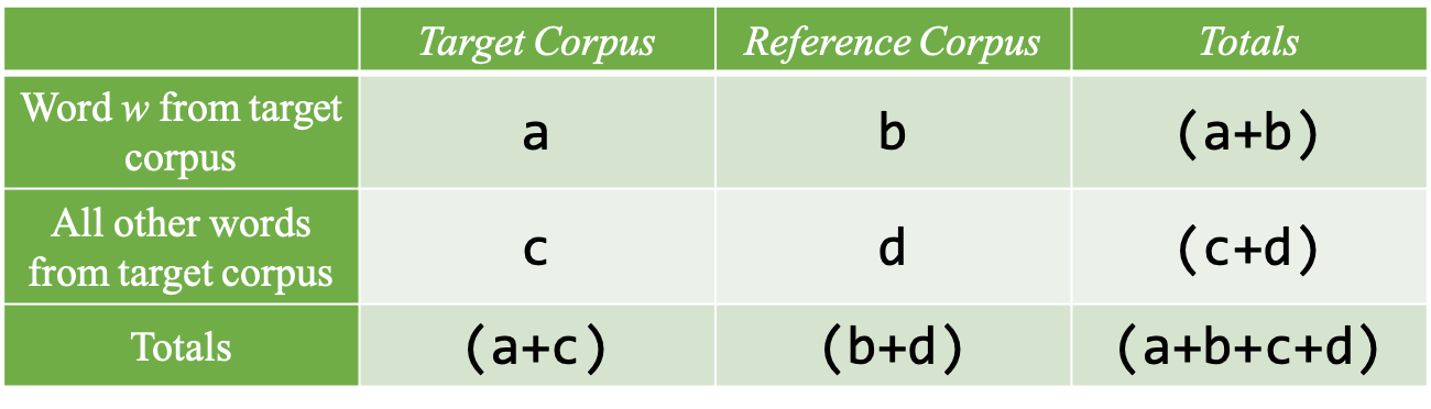
Figure 6.1: Frequency distributions of a word and all other words in two corpora
What are the important factors that may be connected to the significance of the frequencies of the word in two corpora?
- the frequency of the word w in general
- the sizes of the target/reference corpus
In other words, the marginal frequencies of the contingency table are crucial to determining the significance of the word frequencies in two corpora.
Different keyness statistics may have different ways to evaluate the relative importance of the co-occurrences of the word w with the target and the reference corpus (i.e., a and b in Figure 6.1) and statistically determine which connection is stronger.
In this chapter, I would like to discuss three common statistics used in keyness analysis. This tutorial is based on Gries (2017), Ch. 5.2.6.
- Log-likelihood Ratio (G2) (Dunning, 1993);
\[ G^2 = 2 \sum_{i=1}^4 obs \times ln \frac{obs}{exp} \]
- Difference Coefficient (Leech & Fallon, 1992);
\[ difference\;coefficient = \frac{a - b}{a + b} \]
- Relative Frequency Ratio (Damerau, 1993)
\[ rfr = \frac{(a\div b)}{(a+c)\div(b+d)} \]
6.3 Implementation
In this tutorial we will use two documents as our mini reference and target corpus. These two documents are old Wikipedia entries (provided in Gries (2017)) on Perl and Python respectively.
- First we initialize necessary packages in R
- Then we load the corpus data, which are available as two text files in our
demo_data, and transform the corpus into a tidy structure
flist <- c("demo_data/corp_perl.txt", "demo_data/corp_python.txt")
corpus <- readtext(flist) %>%
  corpus %>%
  tidy %>%
  mutate(textid = basename(flist)) %>%
select(textid, text)- We convert the text-based corpus into a word-based data frame, which allows us to easily extract word frequency information
Exercise 6.1 We mentioned this before. It is always good to keep track of the relative positions of the word in the original text. Please create a column in corpus_word, indicating the the relative position of each word in the text with unique word_id.
(NB: Only the first 100 rows are shown here.)
- Now we need to get the frequencies of each word in the two corpora respectively.
- As now we are analyzing each word in relation to the two corpora, it would be better for us to have each word type as one independent row, and columns recording their co-occurrence frequencies with the two corpora (i.e., target and reference).
How to achieve this?
6.4 Tidy Data (Self-Study)
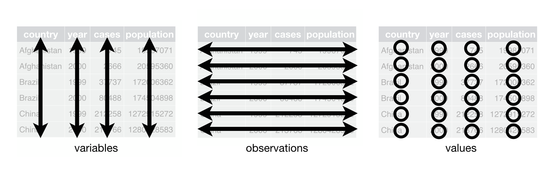
Now I would like to talk about the idea of tidy dataset before we move on. Wickham & Grolemund (2017) suggests that a tidy dataset needs to satisfy the following three interrelated principles:
- Each variable must have its own column.
- Each observation must have its own row.
- Each value must have its own cell.
In our current word_freq, our observation in each row is a word. This is OK because a tidy dataset needs to have every independent word (type) as an independent row in the table.
However, there are two additional issues with our current data frame word_freq:
- Each row in
word_freqin fact represents the combination of two factors, i.e.,word,textid. In addition, the columnncontains the token frequencies for each level combination of these two (nominal) variables. - The same word type appears twice in the dataset in the rows (e.g., the, a)
This is the real life: we often encounter datasets that are NOT tidy at all.
Instead of expecting others to always provide you a perfect tidy dataset for analysis (which is very unlikely), we might as well learn how to deal with messy dataset.
Wickham & Grolemund (2017) suggest two common strategies that data scientists often apply:
Long-to-Wide:
- One variable might be spread across multiple columns
- Create more variables/columns based on one old variable
Wide-to-Long:
- One observation might be scattered across multiple rows
- Reduce several variables/columns by collapsing them into levels of a new variable
6.4.1 An Long-to-Wide Example
Here I would like to illustrate the idea of Long-to-Wide transformation with a simple dataset from Wickham & Grolemund (2017), Chapter 12.
people <- tribble(
  ~name,             ~profile,  ~values,
  #-----------------|--------|------
  "Phillip Woods",   "age",       45,
  "Phillip Woods",   "height",   186,
  "Jessica Cordero", "age",       37,
  "Jessica Cordero", "height",   156
)
people
The above dataset people is not tidy because:
- the column
profilecontains more than one variable; - an observation (e.g., Phillip Woods) is scattered across several rows.
To tidy up people, we can apply the Long-to-Wide strategy:
One variable might be spread across multiple columns
The function tidyr::pivot_wider() is made for this. There are two important parameters in pivot_wider():
names_from = ...: The column from which we create new variable names. Here it’sprofile.values_from = ...: The column from which we take values for new columns. Here it’svalues.
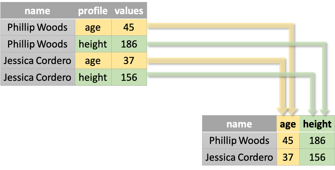
Figure 6.2: From Long to Wide: pivot_wider()
We used pivot_wider() to transform people into a wide-format data frame.
6.4.2 A Wide-to-Long Example
Now let’s take a look at an example of the second strategy, Long-to-Wide transformation.
When do we need this? This type of data transformation is often needed when you see that some of your columns/variables are in fact connected to the same factor.
That is, these columns in fact can be considered levels of another underlying factor.
Take the following simple case for instance.
The dataset preg has three columns: pregnant, male, and female. Of particular interest here are the last two columns. It is clear that male and female can be considered levels of another underlying factor, i.e., gender.
More specifically, the above dataset preg can be tidied up as follows:
- we can have a column
gender - we can have a column
pregnant - we can have a column
count(representing the number of observations for the combinations ofgenderandpregnant)
In other words, we need the Wide-to-Long transformation:
One observation might be scattered across multiple rows.
The function tidyr::pivot_longer() is made for this. There are three important parameters:
cols = ...: The set of columns whose names are levels of an underlying factor. Here they aremaleandfemale.names_to = ...: The name of the new underlying factor. Here it isgender.values_to = ...: The name of the new column for values of level combinations. Here it iscount.
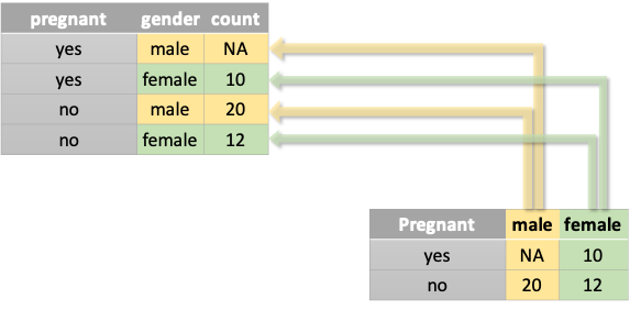
Figure 6.3: From Wide to Long: pivot_longer()
We applied the Wide-to-Long transformation to preg:
6.5 Word Frequency Transformation
Now back to our word_freq:
It is probably clearer to you now what we should do to tidy up word_freq.
- It is obvious that some words (observations) are scattered across several rows.
- The column
textidcan be pivoted into two variables: “perl” vs. “python”.
In order words, we need the data transformation technique of Long-to-Wide.
One variable might be spread across multiple columns
We transformed our data accordingly.
word_freq_wide <- word_freq %>%
  pivot_wider(names_from = "textid",  ## from which original column we gather new variables/colnames
              values_from = "n")      ## from which original column we gather values for new variables

head(word_freq_wide)
Exercise 6.2 In the above Long-to-Wide transformation, there is still one problem. There are quite a few words that occur in one corpus but not the other. For these words, their frequencies would be a NA because R cannot allocate proper values for these unseen cases.
Could you fix this problem by assigning these unseen cases a 0 when transforming the data frame?
Please name the updated wide version of the word frequency data frame as contingency_table.
Hint: Please check the argument pivot_wider(..., values_fill = ...)
- Problematic unseen cases in one of the corpora:
- Updated
contingency_table:
In keyness analysis, words that appear in only one corpus—either the target or the reference—are often the most significant indicators of a sub-language. However, these “unseen” words create a zero-frequency problem in corpus linguistics. Because many association measures rely on division or logarithms, a frequency of zero leads to mathematical errors, such as \(\log(0)\) or division by zero. To resolve this, researchers apply smoothing techniques, such as Laplace Smoothing (or “add-one” smoothing), which adds a small constant to frequency counts to ensure all values remain mathematically tractable.
Before we compute the keyness, we preprocess the data by:
- including words consisting of alphabets only;
- renaming the columns to match the cell labels in Figure 6.1 above;
- creating necessary frequencies (columns) for keyness computation
contingency_table %>%
  filter(word %>% str_detect("^[a-zA-Z]+")) %>%
  rename(a = corp_perl.txt, b = corp_python.txt) %>%
  mutate(c = sum(a)-a, d = sum(b)-b) -> contingency_table

contingency_table
6.6 Computing Keynesss
- With all necessary frequencies, we can now compute the three keyness statistics for each word.
contingency_table %>%
  mutate(a.exp = ((a+b)*(a+c))/(a+b+c+d),
         b.exp = ((a+b)*(b+d))/(a+b+c+d),
         c.exp = ((c+d)*(a+c))/(a+b+c+d),
         d.exp = ((c+d)*(b+d))/(a+b+c+d),
         G2 = 2*(a*log(a/a.exp) + b*log(b/b.exp) + c*log(c/c.exp) + d*log(d/d.exp)),
         DC= (a-b)/(a+b),
         RFR = (a/b)/((a+c)/(b+d))) %>%
  arrange(desc(G2)) %>%
  mutate_if(is.numeric, round, 2) -> keyness_table
keyness_table- Although now we have the keyness values for words, we still don’t know to which corpus (target or reference corpus) the word is more attracted. What to do next?
keyness_table %>%
  mutate(preference = ifelse(a > a.exp, "perl","python")) %>%
  select(word, preference, everything())-> keyness_table

keyness_table
keyness_table %>%
group_by(preference) %>%
top_n(10, G2) %>%
select(preference, word, G2) %>%
arrange(preference, -G2)In his recent work (Gries (2024)), Stefan Gries proposes moving away from traditional p-value-based metrics (like Log-likelihood) in favor of Information Theory. He advocates using Kullback-Leibler (KL) Divergence to measure the “informational surprise” of word distributions. This approach treats keyness as an effect size rather than just statistical significance. I encourage you to explore his “3D Keyness” framework and how \(D_{KL}\) can be used to measure both association and dispersion.
\[ D_{KL}(P \parallel Q) = \sum_{i \in \mathcal{X}} P(i) \log \left( \frac{P(i)}{Q(i)} \right) \]
6.7 Conclusion
Keyness discussed in this chapter is based on the comparative study of word frequencies in two separate corpora: one as the target and the other as the reference corpus. Therefore, the statistical keyness found in the word distribution is connected to the difference between the target and reference corpus (i.e., their distinctive features).
These statistical keywords should be therefore interpreted along with the distinctive feature(s) of the target and reference corpus.
- If the text collections in the target and reference corpus differ significantly in different their time periods, then the keywords may reflect important terms prominent in specific time periods (i.e., diachronic studies).
- If the text collections differ significantly in genres/registers, then the keywords may reflect important terms tied to particular genres/registers.
- If the target corpus is a collection of L2 texts and the reference corpus is a collection of L1 texts, keywords extracted may be indicative of expressions preferred by L1/L2 learners (See Bestgen (2017)).
Please note that the keyness discussed in this chapter is different from the tf.idf (we used in the previous chapter), which is designed to reflect how important a word is to a document in a corpus. tf.idf is more often used in information retrieval. Important words of a document are selected based on the tf.idf weighting scheme; the relevance of the document to the user’s query is determined based on how close the search word(s) is to the important words of the document.
Exercise 6.3 The CSV in demo_data/data-movie-reviews.csv is the IMDB dataset with 50,000 movie reviews and their sentiment tags (source: Kaggle).
The CSV has two columns—the first column review includes the raw texts of each movie review; the second column sentiment provides the sentiment tag for the review. Each review is either positive or negative.
We can treat the dataset as two separate corpora: negative and positive corpora. Please find the top 10 keywords for each corpus ranked by the G2 statistics.
In the data preprocessing, please use the default tokenization in unnest_tokens(..., token = "words"). When computing the keyness, please exclude:
- words that contain at least one non-word symbol in them (e.g. regex class
\W) - words whose frequency is < 10 in either corpus
The expected results are provided below for your reference.
- The first six rows of
demo_data/data-movie-reviews.csv:
- Sample result: