Chapter 5 Parts-of-Speech Tagging

library(tidyverse)
library(tidytext)
library(quanteda)

This chapter uses Python-based packages, which require a properly configured Python environment on your operating system. For more information, please see Python Environment.

This chapter demonstrates how to POS tag a raw-text corpus to identify syntactic categories and explains how to utilize these annotations for sophisticated linguistic analysis.

We will focus on spacyr, an R wrapper for the spaCy Python library, which is widely recognized as an “industrial-strength” tool for natural language processing. Beyond basic POS tagging, this package provides a suite of linguistic annotations essential for in-depth text analysis.

Because spaCy is multilingual, this chapter will also guide you through using spacyr to process both English and Chinese datasets.

We will talk about Chinese text processing in a later chapter, Chinese Text Processing, in a more comprehensive way.

5.1 Installing the Package

Please consult the spacyr GitHub for detailed installation instructions.

The process involves the following steps:

For Python:

Create a Python environment: Set up a dedicated Python environment (such as Miniconda, Anaconda/Conda, Virtual Environments) that you intend to use with R.
Install the Python module: Since spacyr is an R wrapper for the spaCy Python library, you must first install the spacy Python module and its language models (e.g., en_core_web_sm, zh_core_web_sm) in the designated Python environment, using standard Python library installation methods.

It is recommended that you have Python 3.9+ and spacy 3+ at least in your operating system.

We recommend creating your conda environment and installing all necessary Python libraries before returning to R. It is more efficient to install Python’s spacy and its language models directly within the Python conda environment first. Once the environment is configured, you can access and use spacy from R/RStudio by pointing to that specific conda environment.

For R:

Install the spacyr R package:

install.packages("reticulate")
install.packages("spacyr")

Restart R/RStudio and Initialize spaCy in R

Note: I do not recommend this method, as it can occasionally interfere with the default Python environment settings on your operating system.

If you are new to Python and prefer to minimize your direct interaction with it, the simplest approach is to install spaCy through RStudio using the spacyr::spacy_install() function. This function automatically checks for a compatible Python installation on your system; if none is found, it installs one via reticulate::install_python(). It then creates a virtual environment containing all necessary packages in the default directory specified by reticulate::virtualenv_root().

library(spacyr)
spacy_install(version='3.2.4') ## Please note that there are big differences between spacy v2 and v3.

The default settings of spacy_install() is to:

create a stand-alone conda environment including a python executable separate from your system Python (or anaconda python);
install the latest version of spaCy (and its required packages);
download the English language model.

Please check the documentation of spacy_instsall() if you would like to have more specific settings (e.g., spacy version, environment name, python version, language models etc.).

In the following code, we initialize the spacyr Python environment in R using a pre-configured conda environment (e.g., corpling) and the English language model. You can either specify your custom conda environment or virtual environment path, as well as the target language model.

library(spacyr)

## Specify Python Path
Sys.setenv(RETICULATE_PYTHON = "/Users/alvinchen/anaconda3/envs/corpling/bin/python") # needs to point to python binary

## Initialize Spacyr
spacy_initialize(model = "en_core_web_sm")

successfully initialized (spaCy Version: 3.8.2, language model: en_core_web_sm)

R communicates with Python via the library reticulate. If you have installed the library, you can check the current Python path used in the RStudio:

reticulate::py_config()

You can use the reticulate package to identify exactly which Conda environments are available and where they live:

reticulate::conda_list()

## Checking
reticulate::conda_list()

reticulate::py_config() ## check ur python environment

python:         /Users/alvinchen/anaconda3/envs/corpling/bin/python
libpython:      /Users/alvinchen/anaconda3/envs/corpling/lib/libpython3.9.dylib
pythonhome:     /Users/alvinchen/anaconda3/envs/corpling:/Users/alvinchen/anaconda3/envs/corpling
version:        3.9.25 (main, Nov  3 2025, 22:29:32)  [Clang 20.1.8 ]
numpy:          /Users/alvinchen/anaconda3/envs/corpling/lib/python3.9/site-packages/numpy
numpy_version:  2.0.1

NOTE: Python version was forced by RETICULATE_PYTHON

5.2 Quick Overview

5.2.1 Parse the corpus

The spacyr provides a useful function, spacy_parse(), which allows us to parse an English text in a very convenient way.

## naive corpus
txt <- c(d1 = "spaCy is great at fast natural language processing.",
         d2 = "Mr. Smith spent 2.2 years and US$400,000 dollars in N. Carolina.")

## parsing
parsedtxt <- spacy_parse(txt, 
                         pos = T,         # universal POS
                         tag = T,         # OntoNotes 5 POS
                         lemma = T,       # Lemma
                         entity = T,      # Named Entities
                         dependency = T,  # Dependency
                         nounphrase = T)  # NP Chunking

## results
parsedtxt

The output of spacy_parse() is a data frame, which includes token-level annotations of the original texts at multiple levels.

All texts have been tokenized into words with unique IDs (i.e., doc_id, sentence_id, token_id)
The original word form is in the column of token.
The lemma of each word token is provided in lemma.
The POS tag of each word token is provided in pos and tag.
- pos: this column uses the Universal tagset for parts-of-speech, a general POS scheme that suffices most needs, and provides equivalencies across languages
- tag: this column provides a more detailed tagset, defined in each spaCy language model. For English, this is the OntoNotes 5 version of the Penn Treebank tag set (cf. Penn Treebank Tagset)
Depending on the argument setting for spacy_parse(), you can get more annotations, such as named entities (entity) and dependency relations (del_rel).

In SpaCy, the English part-of-speech tagger uses the OntoNotes 5 version of the Penn Treebank tag set. It also maps the tags to the simpler Universal Dependencies v2 POS tag set. The following table shows the descriptions of the tag set.

5.2.2 Quick Analysis

With the output from spacy_parse(), we can perform several analyses right away.

## Entities
entity_extract(parsedtxt)

## NP Chunks
nounphrase_extract(parsedtxt)

## If you haven't installed `rsyntax`
## Uncomment and install
## install.packages("rsyntax")

## Dependency Tree Structure
library(rsyntax)

plot_tree(
  as_tokenindex(parsedtxt),
  doc_id = "d1",
  token,
  lemma,
  pos,
  viewer_size = c(150, 150),
  textsize =1,
  spacing = 2,
  viewer_mode = T
)

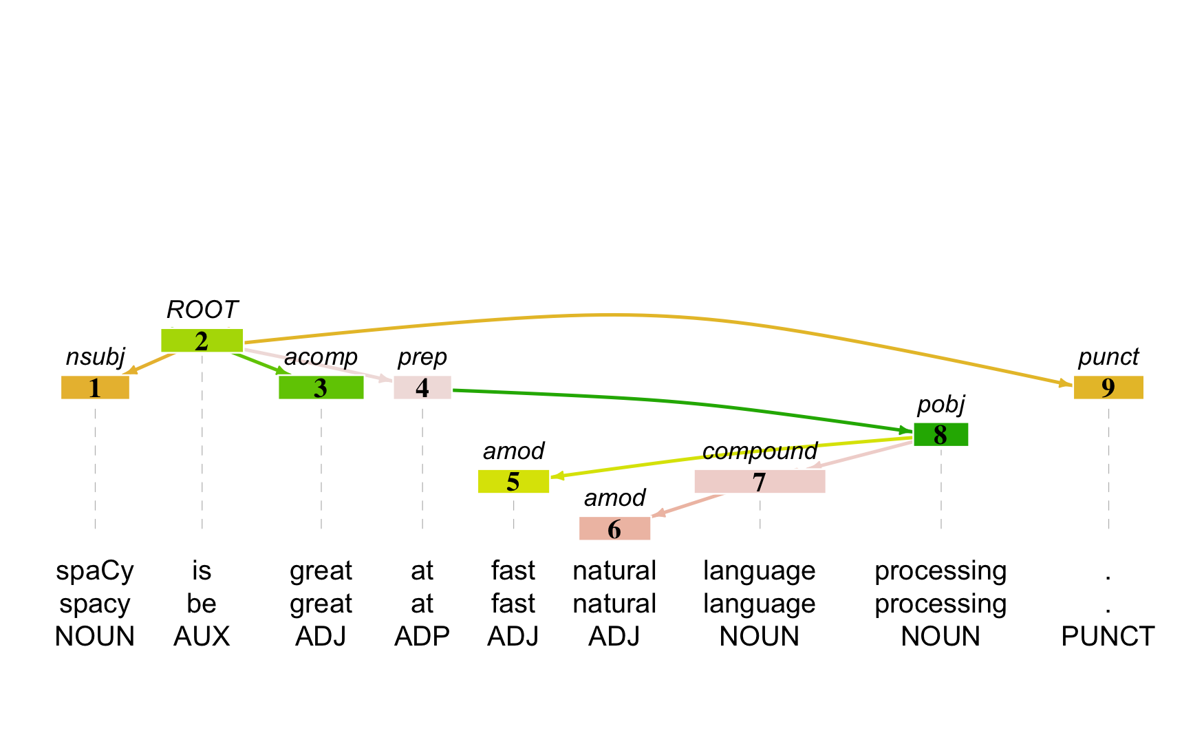
As you can see, with spacy_parse(), you can get a lot of annotations on the corpus data. However, you probably don’t need all of them. So you can specify only those annotations you need from spacy_parse() to save the computing time.

Also, please check the documentation of spacy_parse() for more functions on the parameter additional_attributes =, which allows one to extract additional attributes of tokens from spaCy. For example, additional_attributes = c("like_num", "like_email") gives you whether each token is a number/email or not.

More details on token attributes can be found in spaCy API documentation.

5.3 Working Pipeline

In Chapter 4, we introduced a basic pipeline for text analytics. We now refine this workflow to accommodate different analytical goals (see Figure 5.1).

Once you have secured a collection of raw texts, your choice of path depends on the level of linguistic detail required:

The Right Branch: Follow this workflow if your analysis does not require part-of-speech (POS) tagging or extra syntactic information.
The Left Branch: Follow this workflow if you require the advanced linguistic annotations provided by spacyr.

Figure 5.1: English Text Analytics Flowchart

5.4 Parsing Your Texts

Now let’s use this spacy_parse() to analyze the presidential addresses we’ve seen in Chapter 4: the data_corpus_inaugural from quanteda.

To illustrate the annotation more clearly, let’s parse the first text in data_corpus_inaugural:

library(quanteda)
library(tidytext)

doc1 <- spacy_parse(data_corpus_inaugural[1]) 
doc1

We can parse the whole corpus collection as well. The spacy_parse() can take a character vector as the input, where each element is a text/document of the corpus.

system.time(corp_us_words <- spacy_parse(data_corpus_inaugural))

   user  system elapsed 
  7.350   0.707   8.062

The function system.time() is a useful function which gives you the CPU times that the expression in the parenthesis used. In other words, you can put any R expression in the parenthesis of system.time() as its argument and measure the time required for the expression.

This is sometimes necessary because some of the data processing can be very time consuming. And we would like to know HOW time-consuming it is in case that we may need to run the prodecure again.

corp_us_words

Exercise 5.1 In corpus linguistics analysis, we often need to examine constructions on a sentential level. It would be great if we can transform the word-based data frame into a sentence-based one for more efficient later analysis. Also, on the sentential level, it would be great if we can preserve the information of the lexical POS tags. How can you transform the corp_us_words into one as provided below? (You may name the sentence-based data frame as corp_us_sents.)

5.5 Syntactic Complexity Analysis

Now spacy_parse() has enriched our corpus data with more linguistic annotations. We can now utilize the additional POS tags for more analysis.

In many applied linguistics studies, people sometimes look at the syntactic complexity of the language across a particular factor. For example, people may look at the syntactic complexity development of L2 learners of varying proficiency levels, or of L1 speakers in different acquisition stages, or of writers in different genres (e.g., academic vs. nonacademic).

To operationalize the construct syntactic complexity, we use a simple metric, Fichtner's C, which is defined as:

\[ Fichtner's\;C = \frac{Number\;of\;Verbs}{Number\;of\;Sentences} \times \frac{Number\;of\;Words}{Number\;of\;Sentences} \]

Now we can take the corp_us_words and first generate the frequencies of verbs, and number of words for each presidential speech text.

syn_com <- corp_us_words %>%  ## our word-based DF
  group_by(doc_id) %>% ## for each doc
  summarize(verb_num = sum(pos=="VERB"),  ## calculate total number of verbs
            sent_num = max(sentence_id),  ## calculate total number of sents
            word_num = n()) %>%           ## calculate total num of words
  mutate(F_C = (verb_num/sent_num)*(word_num/sent_num)) %>%   ## Compute C
  ungroup

syn_com

With the syntactic complexity of each president, we can plot the tendency:

syn_com %>%
  ggplot(aes(x = doc_id, y = F_C, fill = doc_id)) + 
  geom_col() + 
  theme(axis.text.x = element_text(angle=90)) +
  labs(title = "Syntactic Complexty", x = "Presidents", y = "Fichtner's C") +
  guides(fill = "none")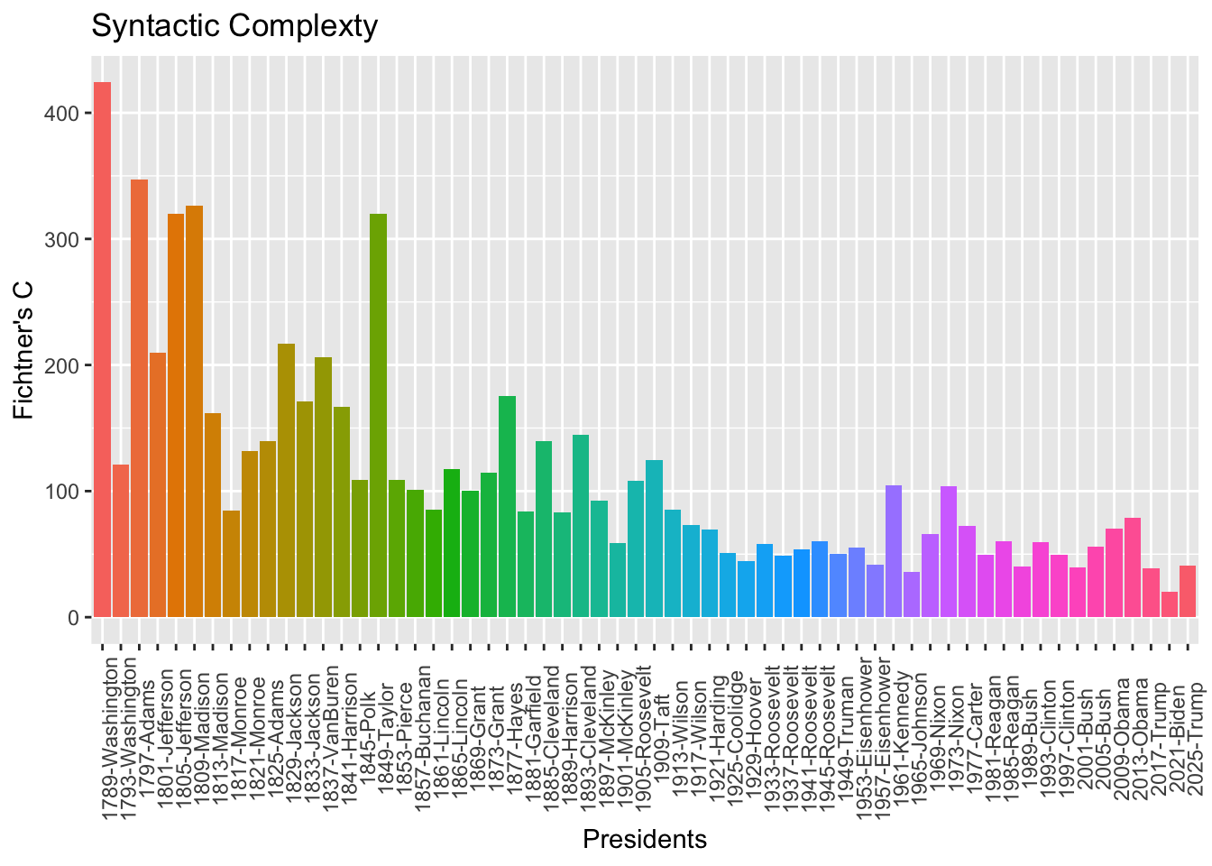

It’s interesting to see a decreasing trend in syntactic complexity!

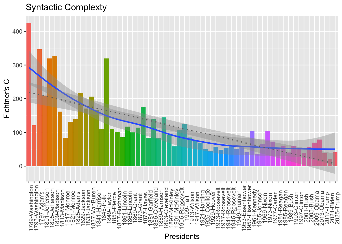
Exercise 5.2 Please add a regression/smooth line to the above plot to indicate the downward trend?

Exercise 5.3 Extract all the subject-predicate word token pairs from the corpus of the presidential addresses. This relationship is defined as a syntactic dependency relationship of nsubj between two word tokens. The subject token is the dependent and the predicate token is the head.

The output includes the subject-predicate token pairs and their relevant information (e.g., From which sentence of which presidential address is the pair extracted?)

Please ignore the tagging errors made by the dependency parser in spacyr.

5.6 Construction Analysis

Now with parts-of-speech tags, we are able to look at more linguistic patterns or constructions in detail. These POS tags allow us to extract more precisely the target patterns we are interested in.

In this section, we will use the output from Exercise 5.1. We assume that now we have a sentence-based corpus data frame, corp_us_sents. Here I like to provide a case study on English Preposition Phrases.

## ######################################
## If you haven't finished the exercise, 
## the dataset is also available in 
## `demo_data/corp_us_sents.RDS
## ######################################

## Uncomment this line if you dont have `corp_us_sents`
# corp_us_sents <- readRDS("demo_data/corp_us_sents.RDS") 

corp_us_sents

We can utilize the regular expressions to extract PREP + NOUN combinations from the corpus data.

## define regex patterns
pattern_pat1 <- "[^/ ]+/ADP [^/]+/NOUN"

## extract patterns from corp
corp_us_sents %>%
  unnest_tokens(
    output = pat_pp,
    input = sentence_tag,
    token = function(x)
      str_extract_all(x, pattern = pattern_pat1)
  ) -> result_pat1

result_pat1

In the above example, we specify the token= argument in unnest_tokens(..., token = ...) with a self-defined (anonymous¹) function.

The idea of tokenization with unnest_tokens() is that the token argument can be any function which takes a text-based vector as input (i.e, each element of the input vector is a document string) and returns a list, each element of which is a token-based version (i.e., vector) of the original input vector element (cf. Figure 5.2).

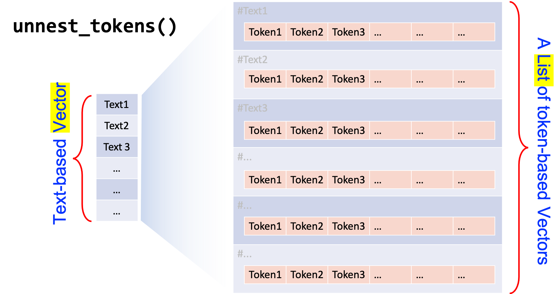
Figure 5.2: Intuition for token= in unnest_tokens()

In the above example, we define a tokenization function:

## verbose format
function(x) {
      str_extract_all(x, pattern = pattern_pat1)
}

## simpler format 
function(x) str_extract_all(x, pattern = pattern_pat1)

This function takes a vector, sentence_tag, as the input and returns a list, each element of which consists a vector of tokens matching the regular expressions from each sentence in sentence_tag.

(Note: The function object is not assigned to an object name, thus never being created in the R working session.)

Exercise 5.4 Create a new column, pat_clean, with all annotations removed in the data frame result_pat1.

With these constructional tokens of English PP’s, we can then do further analysis.

We first identify the PREP and NOUN for each constructional token.
We then clean up the data by removing POS annotations.

## extract the prep and head
result_pat1 %>%
  tidyr::separate(col="pat_pp", into=c("PREP","NOUN"), sep="\\s+" ) %>%
  mutate(PREP = str_replace_all(PREP, "/[^ ]+",""),
         NOUN = str_replace_all(NOUN, "/[^ ]+","")) -> result_pat1a
result_pat1a

Now we are ready to explore the text data.

We can look at how each preposition is being used by different presidents:

result_pat1a %>%
  count(doc_id, PREP) %>%
  arrange(doc_id, desc(n))

We can examine the most frequent NOUN that co-occurs with each PREP:

# Most freq NOUN for each PREP
result_pat1a %>%
  count(PREP, NOUN) %>%
  group_by(PREP) %>%
  top_n(1,n) %>%
  arrange(desc(n))

We can also look at a more complex usage pattern: how each president uses the PREP of in terms of their co-occurring NOUNs?

# NOUNS for `of` uses across different presidents
result_pat1a %>%
  filter(PREP == "of") %>%
  count(doc_id, PREP, NOUN) %>%
  tidyr::pivot_wider(
    id_cols = c("doc_id"),
    names_from = "NOUN",
    values_from = "n",
    values_fill = list(n=0))

Exercise 5.5 In our earlier demonstration, we made a naive assumption: Preposition Phrases include only those cases where PREP and NOUN are adjacent to each other. But there are many more tokens where words do come between the PREP and the NOUN (e.g., with greater anxieties, by your order).

Please revise the regular expression to improve the retrieval of the English Preposition Phrases from the corpus data corp_us_sents.

Specifically, we can define an English PP as a sequence of words, which start with a preposition, and end at the first word after the preposition that is tagged as NOUN, PROPN, or PRON.

The following table shows a sample of the outputs.

Exercise 5.6 Based on the output from Exercise 5.5, please identify the PREP and NOUN for each constructional token and save information in two new columns.

5.7 Issues on Pattern Retrieval

Any automatic pattern retrieval comes with a price: there are always errors returned by the system.

I would like to discuss this issue based on the second text, 1793-Washington. First let’s take a look at the Preposition Phrases extracted by my regular expression used in Exercise 5.5 and 5.6:

## ######################################
## If you haven't finished the exercise, 
## the dataset is also available in
## `demo_data/result_pat2a.RDS
## ######################################

## uncomment this line if you dont have `result_pat2a`
# result_pat2a <- readRDS("demo_data/result_pat2a.RDS") 

result_pat2a %>%
  filter(doc_id == "1793-Washington")

My regular expression has identified 19 PP’s from the text. However, if we go through the text carefully and do the PP annotation manually, we may have different results.

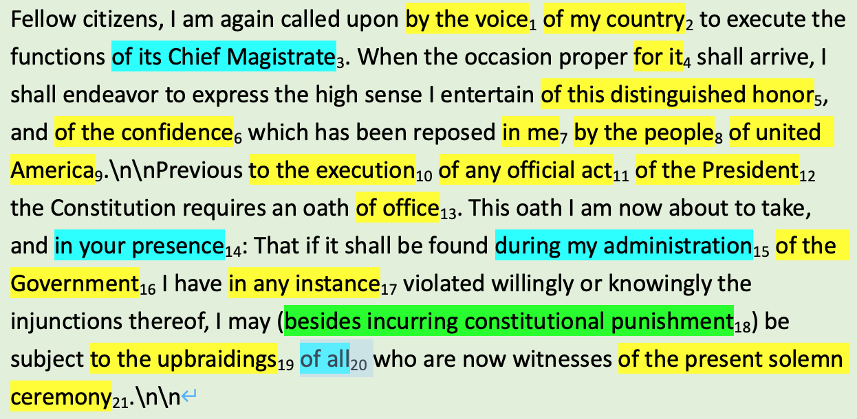
Figure 5.3: Manual Annotation of English PP’s in 1793-Washington

There are two types of errors (cf. x in Figure 5.3):

False Positives: Patterns identified by the system (i.e., regular expression) but in fact they are not true patterns
False Negatives: True patterns in the data but are not successfully identified by the system

As shown in Figure 5.3, manual annotations have identified 20 PP’s from the text while the regular expression identified 19 tokens. A comparison of the two results shows that:

In the regex results, the five highlighted tokens (rows in pink) are False Positives. While the regular expression flagged them as PPs, manual annotation confirms that they do not belong to this category.

pat_pp	PREP	NOUN	doc_id	sentence_id	row_id
by/adp the/det voice/noun	by	voice	1793-Washington	1	1
of/adp my/pron	of	my	1793-Washington	1	2
of/adp its/pron	of	its	1793-Washington	1	3
of/adp this/det distinguished/adj honor/noun	of	honor	1793-Washington	2	4
of/adp the/det confidence/noun	of	confidence	1793-Washington	2	5
in/adp me/pron	in	me	1793-Washington	2	6
by/adp the/det people/noun	by	people	1793-Washington	2	7
of/adp united/propn	of	united	1793-Washington	2	8
to/adp the/det execution/noun	to	execution	1793-Washington	3	9
of/adp any/det official/adj act/noun	of	act	1793-Washington	3	10
of/adp the/det president/propn	of	president	1793-Washington	3	11
of/adp office/noun	of	office	1793-Washington	3	12
in/adp your/pron	in	your	1793-Washington	4	13
during/adp my/pron	during	my	1793-Washington	4	14
of/adp the/det government/propn	of	government	1793-Washington	4	15
in/adp any/det instance/noun	in	instance	1793-Washington	4	16
to/adp the/det upbraidings/noun	to	upbraidings	1793-Washington	4	17
of/adp all/pron	of	all	1793-Washington	4	18
of/adp the/det present/adj solemn/adj ceremony/noun	of	ceremony	1793-Washington	4	19

In the manual annotation shown in Figure 5.3, there are six primary errors. In addition to the five PPs where the NP heads were misidentified, one specific PP (besides incurring constitutional punishment) was missed entirely. The current regex query incorrectly categorized this instance as a negative result, making it a False Negative.

In text processing, it is essential to cultivate a debugging mindset. When your code fails to capture a target (such as the false negative besides incurring constitutional punishment), the most important step isn’t just to try another pattern; it’s to diagnose exactly why the failure occurred.

Rather than guessing at a new solution, what practical steps can you take to identify the specific gap in your current regular expression’s coverage?

We can summarize the pattern retrieval results as:

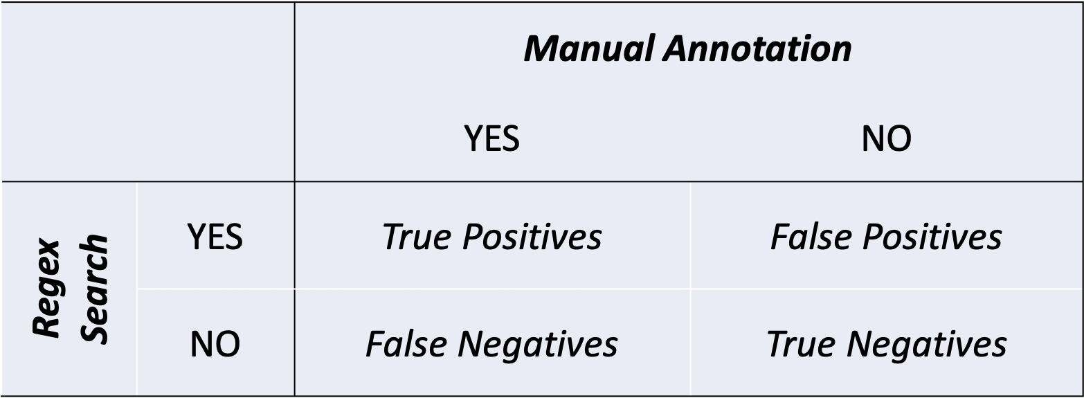
Most importantly, we can describe the quality/performance of the pattern retrieval with two important measures.

\(Precision = \frac{True\;Positives}{True\;Positives + False\;Positives}\) (among all the regex’s positives, how many of them are true positives?)
\(Recall = \frac{True\;Positives}{True\;Positives + False\;Negatives}\) (among all the correct positives, how many of them are correctly retrieved as positives?)

In our case:

\(Precision = \frac{14}{14+5} = 73.68%\)
\(Recall = \frac{14}{14+6} = 70.00%\)

It is rarely possible to achieve 100% precision or recall when automatically retrieving linguistic patterns. Consequently, researchers must often find a strategic compromise between manual accuracy and computational scale.

The following heuristics, based on my experience, can help guide your annotation strategy:

Small Datasets: Manual annotation remains the gold standard, as it provides the highest level of accuracy for limited data.
Moderate Datasets: A semi-automatic approach is often most efficient. Use automated tools for the initial pass, then perform a manual “sanity check” to correct systematic errors.
Large Datasets: Fully automatic annotation is preferred to capture broad linguistic tendencies. However, you should always evaluate the system’s effectiveness by manually checking a random, representative sample of the data.
Complex Semantics: The more an annotation relies on deep meaning—such as conceptual metaphors, sense distinctions, or dialogue acts—the more likely it is to require manual coding or human-in-the-loop verification.
Standard Structural Annotations: Tasks such as Chinese word segmentation, POS tagging, named entity recognition, and dependency parsing are well-suited for fully automatic pipelines.
The AI/LLM Alternative: For tasks that sit between simple POS tagging and complex manual coding, Large Language Models (LLMs) can be leveraged. AI-assisted annotation can handle complex semantic tasks with higher consistency than simple pattern matching while maintaining much greater speed than human coders.

In medicine, there are two similar metrics used for the assessment of the diagnostic medical tests—sensitivity (靈敏度) and specificity (特異性).

Sensitivity refers to the proportion of true positives that are correctly identified by the medical test. This is indeed the recall rates we introduced earlier.
\(Sensitivity = \frac{True\;Positives}{True\;Positives + False\;Negatives}\)
Specificity refers to the proportion of true negatives that are correctly identified by the medical test. It is computed as follows:
\(Specificity = \frac{True\;Negatives}{False\;Positives + True\;Negatives}\)

In plain English, Sensitivity measures the ability of a test to correctly identify those with the disease (the true positive rate); Specificity measures the ability of a test to correctly identify those without the disease (the true positive rate).

Take the pandemic COVID19 for example. If one aims to develop an effective antigen rapid test for COVID19, which metric would be a more reliable and crucial evaluation metric for the quality of the test?

Exercise 5.7 Please extract all English preposition phrases from the presidential addresses by making use of the dependency parsing provided in spacyr.

Also, please discuss whether this dependency-based method improves the quality of pattern retrieval with the 1793-Washington text as an example. In particular, please discuss the precision and recall rates of the dependency-based method and our previous POS-based method.

Dependency-based results on 1793-Washington are provided below.

5.8 Saving POS-tagged Texts

We may very often get back to our corpus texts again and again when we explore the data. In order NOT to re-tag the texts every time we analyze the data, it would be more convenient if we save the tokenized texts with the POS tags in external files. Next time we can directly load these files without going trough the POS-tagging again.

However, when saving the POS-tagged results to an external file, it is highly recommended to keep all the tokens of the original texts. That is, leave all the word tokens as well as the non-word tokens intact.

A few suggestions:

If you are dealing with a small corpus, I would probably suggest you to save the resulting data frame from spacy_parse() as a csv for later use.
If you are dealing with a big corpus, I would probably suggest you to save the parsed output of each text file in an independent csv for later use.

write_csv(corp_us_words, "corp-inaugural-word.csv")

5.9 Finalize spaCy

While running spaCy on Python through R, a Python process is always running in the background and R session will take up a lot of memory (typically over 1.5GB).

spacy_finalize() terminates the Python process and frees up the memory it was using.

spacy_finalize()

Also, if you would like to use other spacy language models in the same R session, or change the default Python environment in the same R session, you can first use spacy_finalize() to quit from the current Python environment.

5.10 Notes on Chinese Processing

The library spacyr supports Chinese processing as well. The key is you need to download the Chinese language model from the original spaCy and make sure that the language model is accessible in the python environment you are using in R.

############################
### Chinese Processing    ##
############################

library(spacyr)
spacy_initialize(model = "zh_core_web_sm")
reticulate::py_config() ## check ur python environment

python:         /Users/alvinchen/anaconda3/envs/corpling/bin/python
libpython:      /Users/alvinchen/anaconda3/envs/corpling/lib/libpython3.9.dylib
pythonhome:     /Users/alvinchen/anaconda3/envs/corpling:/Users/alvinchen/anaconda3/envs/corpling
version:        3.9.25 (main, Nov  3 2025, 22:29:32)  [Clang 20.1.8 ]
numpy:          /Users/alvinchen/anaconda3/envs/corpling/lib/python3.9/site-packages/numpy
numpy_version:  2.0.1

NOTE: Python version was forced by RETICULATE_PYTHON

txt_ch <- c(d1 = "2022年1月7日 週五 上午4:42·1 分鐘 (閱讀時間)
桃園機場群聚感染案件確診個案增，也讓原本近日展開的尾牙餐會受到波及，桃園市某一家飯店不斷接到退訂，甚至包括住房、圍爐等，也讓飯店人員感嘆好不容易看見有點復甦景象，一下子又被疫情打亂。（李明朝報導）",
         d2 = "桃園機場群聚感染，隨著確診個案增加，疫情好像短時間無法終結，原本期待在春節期間能夠買氣恢復的旅宿業者，首當其衝大受波及，桃園市一家飯店人員表示，「1月6日就開始不斷接到消費者打來電話，包括春酒尾牙、圍爐桌席和住房，其中單單一個上午就有約20桌宴席、近百間房取消或延期。")
parsedtxt_ch <- spacy_parse(txt_ch, 
                         pos = T, 
                         tag = T, 
                         # lemma = T,
                         entity = T,
                         dependency = T)


parsedtxt_ch

With the enriched information of the text, we can perform more in-depth exploration of the text. For example, identify useful semantic information from the named entities in the text.

## Extract named entities (dates, events, and cardinal or ordinal quantities)
entity_extract(parsedtxt_ch, type="all")

## Compound multiword entities into single tokens
entity_consolidate(parsedtxt_ch)

spacy_finalize()

5.11 Useful Information

In order to make good use of all the functionalities provided by spacy, one may need to have clearer understanding of all the annotations and the meanings of the tags at different linguistic levels (e.g., POS tags, Universal POS Tags, Dependency Tags etc.). Most importantly, the tag sets may vary from language to language.

For more detail, please refer to this glossary.py from the original spacy module.

In general, here are a few common annotation schemes:

Universal POS Tags
POS Tags (Chinese): OntoNotes Chinese Penn Treebank
POS tags (English): OntoNotes 5 Penn Treebank
Dependency Labels (English): ClearNLP / Universal Dependencies
Named Entity Recognition: OntoNotes 5

Exercise 5.8 Use the script of PTT Crawler you created in the previous chapter and collect your corpus data from the Gossiping Board. With your corpus data collected, please present the corpus size in terms of word numbers.

Also, please create a word cloud for your corpus by including only disyllabic words whose parts of speech fall into the following categories: nouns and verbs.

Exercise 5.9 In this exercise, please use the corpus data provided in quanteda.textmodels::data_corpus_moviereviews. This dataset is provided as a corpus object in the package quanteda.textmodels (please install the package on your own). The data_corpus_moviereviews includes 2,000 movie reviews.

Please use the spacyr to parse the texts and provide the top 20 adjectives for positive and negative reviews respectively. Adjectives are naively defined as any words whose pos tags start with “J” (please use the fine-grained version of the POS tags. i.e., tag, from spacyr). When computing the word frequencies, please use the lemmas instead of the word forms.
Please provide the top 20 words that are content words for positive and negative reviews ranked by a weighted frequency score, which is computed using the formula provided below (See the info box below for more explanation). Content words are naively defined as any words whose pos tags start with N, V, or J.

(In my results below, there is one additional criterion for word selection: words whose first letter starts with a non-alphanumeric character are removed from the frequency list.)

\[Word\;Frequency \times log(\frac{Numbe\; of \; Documents}{Word\;Diserpsion}) \]

For example, if the lemma action occurs 691 times in the negative reviews collection. These occurrences are scattered in 337 different documents. There are 1000 negative texts in the current corpus. Then the weighted score for action is:

\[691 \times log(\frac{1000}{337}) = 751.58 \]

summary(quanteda.textmodels::data_corpus_moviereviews)

ans1

ans2

In our earlier chapters, we have discussed the issues of word frequencies and their significance in relation to the dispersion of the words in the entire corpus. In terms of identifying important words from a text collection, our assumption is that: if a word is scattered in almost every document in the corpus collection, it is probably less informative. For example, words like a, the would probably be observed in every document in the corpus. Therefore, the high frequencies of these widely-dispersed words may not be as important compared to the high frequencies of those which occur in only a subset of the corpus collection. The word frequency is sometimes referred to as term frequency (tf) in information retrieval; the dispersion of the word is referred to as document frequency (df). In information retrieval, people often use a weighting scheme for word frequencies in order to extract informative words from the text collection. The scheme is as follows:

\[tf \times log(\frac{N}{df}) \]

N refers to the total number of documents in the corpus. The \(log\frac{N}{df}\) is referred to as inversed document frequency (idf). This tf.idf weighting scheme is popular in many practical applications.

The smaller the df of a word, the higher the idf, the larger the weight for its tf.

It is an anonymous function because it has not be defined with an object name in the R session.↩︎