Chapter 8 Constructions and Idioms
library(tidyverse)
library(tidytext)
library(quanteda)
library(stringr)
library(jiebaR)
library(readtext)
8.1 Collostructional Analysis: An Introduction
Collostructional analysis is a family of quantitative methods developed within Construction Grammar (CxG) to measure the statistical association between specific lexical items and the grammatical constructions they inhabit. Introduced primarily by Stefan Gries and Anatol Stefanowitsch in the early 2000s, it moves beyond simple word-level collocations to examine “lexico-grammatical” preferences.
Instead of just looking at word-to-word associations, these methods use statistical measures (e.g., Fisher’s Exact Test or Log-likelihood, Kullback-Leibler Divergence) to determine if a word occurs in a construction significantly more (or less) often than expected by chance.
8.1.1 The Four Main Methods
- Collexeme Analysis: Measures the association between a single construction and the words (collexemes) that fill a specific slot (e.g., which verbs are most “attracted” to the Ditransitive Construction).
- Distinctive Collexeme Analysis: Compares two near-synonymous constructions to see which words prefer one over the other (e.g., comparing the Ditransitive vs. Prepositional Dative).
- Covarying Collexeme Analysis: Examines the relationship between two different slots within the same construction (e.g., the relationship between the verb and the V-ing in the V-into-Ving construction: fool into thinking, mislead into believing).
- Multiple Distinctive Collexeme Analysis: An extension used to compare three or more alternating constructions.
8.1.2 Important Studies and Foundations
- Stefanowitsch & Gries (2003): The seminal paper that introduced Collexeme Analysis, demonstrating how the “meaning” of a construction can be empirically derived from the words that most frequently fill in a specific slot of the construction.
- Gries & Stefanowitsch (2004): This study introduced Distinctive Collexeme Analysis, proving that near-synonymous constructions (like the dative alternation) have subtle semantic differences based on the verbs they attract.
- Stefanowitsch & Gries (2005): This study introduced Covarying Collexeme Analysis, showing how the study of two words occupying the slots of the construction reveals the constructional semantic coherences/regularities.
- Hilpert (2008): Applied these methods to Diachronic (historical) Linguistics, showing how the lexical preferences of constructions change over time, a process known as diachronic collostructional analysis.
- Gries (2024): Recent work by Gries refines these metrics by prioritizing effect size and information theory (specifically KL Divergence) over traditional p-values. This approach aims to minimize common statistical pitfalls, such as the tendency for frequency to confound traditional measures of associations.
In this chapter, I will demonstrate how we can conduct collostructional analysis by using the R script written by Stefan Gries (Collostructional Analysis).
8.2 Corpus
In this chapter, I will use the Apple News Corpus from Chapter 7 as our corpus. (It is available in: demo_data/applenews10000.tar.gz.)
And in this demonstration, I would like to look at a particular morphosyntactic frame in Chinese, X + 起來. Our goal is simple: in order to find out the semantics of this constructional schema, it would be very informative if we can find out which words tend to strongly occupy this X slot of the constructional schema.
That is, we are interested in the collexemes of the construction X + 起來 and their degree of semantic coherence.
So our first step is to load the text collections of Apple News into R and create a corpus object.
## Text normalization function
## Define a function
normalize_document <- function(texts) {
  texts %>%
    str_replace_all("\\p{C}", " ") %>%  ## remove control chars
    str_replace_all("\\s+", "\n")  ## replace whitespaces with linebreak
}

## Load Data
apple_df <-
  readtext("demo_data/applenews10000.tar.gz", encoding = "UTF-8") %>% ## loading data
  filter(!str_detect(text, "^\\s*$")) %>% ## removing empty docs
mutate(doc_id = row_number()) ## create index[1] "《蘋果體育》即日起進行虛擬賭盤擂台,每名受邀參賽者進行勝負預測,每周結算在周二公布,累積勝率前3高參賽者可繼續參賽,單周勝率最高者,將加封「蘋果波神」頭銜。註:賭盤賠率如有變動,以台灣運彩為主。\n資料來源:NBA官網http://www.nba.com\n\n金塊(客) 103:92 76人騎士(主) 88:82 快艇活塞(客) 92:75 公牛勇士(客) 108:82 灰熊熱火(客) 103:82 灰狼籃網(客) 90:82 公鹿溜馬(客) 111:100 馬刺國王(客) 112:102 爵士小牛(客) 108:106 拓荒者\n\n"[1] "《蘋果體育》即日起進行虛擬賭盤擂台,每名受邀參賽者進行勝負預測,每周結算在周二公布,累積勝率前3高參賽者可繼續參賽,單周勝率最高者,將加封「蘋果波神」頭銜。註:賭盤賠率如有變動,以台灣運彩為主。\n資料來源:NBA官網http://www.nba.com\n金塊(客)\n103:92\n76人騎士(主)\n88:82\n快艇活塞(客)\n92:75\n公牛勇士(客)\n108:82\n灰熊熱火(客)\n103:82\n灰狼籃網(客)\n90:82\n公鹿溜馬(客)\n111:100\n馬刺國王(客)\n112:102\n爵士小牛(客)\n108:106\n拓荒者\n"Raw texts usually include a lot of noise. For example, texts may include invisible control characters, redundant white-spaces, and duplicate line breaks. These redundant characters may have an impact on the word segmentation performance. It is often suggested to clean up the raw texts before tokenization.
In the above example, I created a simple function, normalize_text(). You can always create a more sophisticated one that is designed for your own corpus data.
8.3 Word Segmentation
We use the self-defined word tokenization method based on jiebar. There are three important steps:
- We first initialize a
jiebarlanguage model usingworker(); - We then define a function
word_seg_text(), which enriches the raw texts with word boundaries and parts-of-speech tags; - Then we apply the function
word_seg_text()to the original texts and create a new column to our text-based data frame, a column with the enriched versions of the original texts.
This new column will serve as the basis for later construction extraction.
# Initialize jiebar
segmenter <- worker(user = "demo_data/dict-ch-user.txt",
                    bylines = F,
                    symbol = T)

# Define function
word_seg_text <- function(text, jiebar) {
  segment(text, jiebar) %>% # word tokenize
    str_c(collapse = " ") ## concatenate word tokens into long strings
}

# Apply the function
apple_df <- apple_df %>%
  mutate(text_tag = map_chr(text, word_seg_text, segmenter))
Our self-defined function word_seg_text() is a simple function to convert a Chinese raw text into am enriched version with word boundaries and POS tags.
[1] "《 蘋果 體育 》 即日起 進行 虛擬 賭盤 擂台 , 每名 受邀 參賽者 進行 勝負 預測 , 每周 結算 在 周二 公布 , 累積 勝率 前 3 高 參賽者 可 繼續 參賽 , 單周 勝率 最高者 , 將 加封 「 蘋果 波神 」 頭銜 。 註 : 賭盤 賠率 如有 變動 , 以 台灣 運彩 為主 。 \n 資料 來源 : NBA 官網 http : / / www . nba . com \n 金塊 ( 客 ) \n 103 : 92 \n 76 人 騎士 ( 主 ) \n 88 : 82 \n 快艇 活塞 ( 客 ) \n 92 : 75 \n 公牛 勇士 ( 客 ) \n 108 : 82 \n 灰熊 熱火 ( 客 ) \n 103 : 82 \n 灰狼 籃網 ( 客 ) \n 90 : 82 \n 公鹿 溜 馬 ( 客 ) \n 111 : 100 \n 馬刺 國王 ( 客 ) \n 112 : 102 \n 爵士 小牛 ( 客 ) \n 108 : 106 \n 拓荒者 \n"Please note that in this example, we did not include the parts-of-speech tagging in order to keep this example as simple as possible. However, in real studies, we often need to rely on the POS tags if we want to improve the quality of the pattern retrieval.
Therefore, for your own project, probably you need to revise the word_seg_text() and also the jiebar language model (worker()) if you would like to include the POS tag annotation in the data processing.
Also, due to the heavier computational cost of POS tagging, maybe you can consider splitting text into smaller chunks (e.g., lines, sentences) first before segmentation processing.
8.4 Collexeme Analysis
8.4.1 Extract Constructions
With the word boundary information, we can now extract our target patterns from the corpus using regular expressions with unnest_tokens().
# Define regex
pattern_qilai <- "[^\\s]+\\s起來\\b"

# Extract patterns
apple_qilai <- apple_df %>%
  select(-text) %>% ## dont need original texts
  unnest_tokens(
    output = construction, ## name for new unit
    input = text_tag, ## name of old unit
    token = function(x) ## unesting function
      str_extract_all(x, pattern = pattern_qilai)
  )

# Print
apple_qilai
8.4.2 Distributional Information Needed for CA
To perform the collexeme analysis, which is essentially a statistical analysis of the association between words and a specific construction, we need to collect necessary distributional information of the words (X) and the construction (X + 起來).
In particular, to use Stefan Gries’ R script of Collostructional Analysis, we need the following information:
- Co-occurring Frequencies of the words and the construction
- Frequencies of Words in Corpus
- Corpus Size (total number of words in corpus)
Take the word 使用 for example. We need the following distributional information:
- Co-occurring Frequencies: the frequency of
使用+起來 - The frequency of
使用in Corpus - Corpus Size (total number of words in corpus)
8.4.2.1 Collecting Word Frequency
Let’s attend to the second distributional information needed for the analysis : the frequencies of words/collexemes.
It is easy to get the word frequencies of the entire corpus.
With the tokenized texts, we first convert the text-based data frame into a word-based one; then we create the word frequency list via simple data manipulation tricks.
## create word freq list
apple_word_freq <- apple_df %>%
  select(-text) %>% ## dont need original raw texts
  unnest_tokens( ## tokenization
    word,  ## new unit
    text_tag,  ## old unit
    token = function(x)  ## tokenization function
      str_split(x, "\\s+")
  ) %>%
  filter(nzchar(word)) %>% ## remove empty strings
  count(word, sort = T)

apple_word_freq %>%
  head(100)
In the above example, when we convert our data frame from a text-based to a word-based one, we didn’t use any specific tokenization function in unnest_tokens() because we have already obtained the enriched version of the texts, i.e., texts where each word token is delimited by a white-space. Therefore, the unnest_tokens() here is a lot simpler: we simply tokenize the texts into word tokens based on the known delimiter, i.e., the white-spaces.
8.4.2.2 Collecting Joint Frequencies
Now let’s attend to the first distributional information needed for the analysis: the joint frequencies of X and the QILAI-construction.
With the earlier pattern-based data frame, apple_qilai, this should be simple. Also, because we have created the word frequency list of the corpus, we can include the corpus frequency of X in the same data frame as well.
## Joint frequency table
apple_qilai_freq <- apple_qilai %>%
  count(construction, sort = T) %>%  ## get joint frequencies
  tidyr::separate(col = "construction", ## restructure data frame
                  into = c("w1", "construction"),
                  sep = "\\s") %>%
  ## identify the freq of X in X_起來
  mutate(w1_freq = apple_word_freq$n[match(w1, apple_word_freq$word)])

apple_qilai_freq
8.4.2.3 Preparing Data Input File
The script coll.analysis.r expects a particular input format.
The input file should be a tsv file, which includes a three-column table:
- Words
- Word frequency in the corpus
- Word joint frequency with the construction
## prepare a tsv
## for coll analysis
apple_qilai_freq %>%
  select(w1, w1_freq, n) %>%
  write_tsv("qilai.tsv")
In the later Stefan Gries’ R script, it requires that the input be a tab-delimited file (tsv), not a comma-delimited file (csv).
8.4.2.4 Collecting Corpus Size
In addition to the input file, Stefan Gries’ coll.analysis.r also requires a few general statistics for the computing of association measures.
We prepare necessary distributional information for the later collostructional analysis:
- Corpus size: The total number of words in the corpus
- Construction size: the total number of the construction tokens in the corpus
Later when we run Gries’ script, we need to enter these numbers manually in the terminal.
Corpus Size: 3209784 Construction Size: 546 Collexeme Candidate Types: 200Sometimes you may need to keep important information printed in the R console in an external file for later use. There’s a very useful function, sink(), which allows you to easily keep track of the outputs printed in the R console and save these outputs in an external text file.
## save info in a text
sink("qilai_info.txt") ## start flushing outputs to the file not the terminal
cat("Corpus Size: ", sum(apple_word_freq$n), "\n")
cat("Construction Size: ", sum(apple_qilai_freq$n), "\n")
cat("Collexeme Candidate Types: ", nrow(apple_qilai_freq))
sink() ## end flushing
You should be able to find a newly created file, qilai_info.txt, in your working directory, where you can keep track of the progress reports of your requested information.
Therefore, sink() is a useful function that helps you direct necessray terminal outputs to an external file for later use.
8.4.3 Running Collostructional Analysis
We are now ready to run the analysis by sourcing coll.analysis.r, available on Stefan Gries’ website.
We can use source() to run the entire R script. The coll.analysis.r is available on Stefan Gries’ website. We can either save the script onto our laptop and run it offline or source the online version ( coll.analysis.r) directly.
######################################
## WARNING!!!!!!!!!!!!!!! ##
## The script re-starts a R session ##
######################################
source("https://www.stgries.info/teaching/groningen/coll.analysis.r")
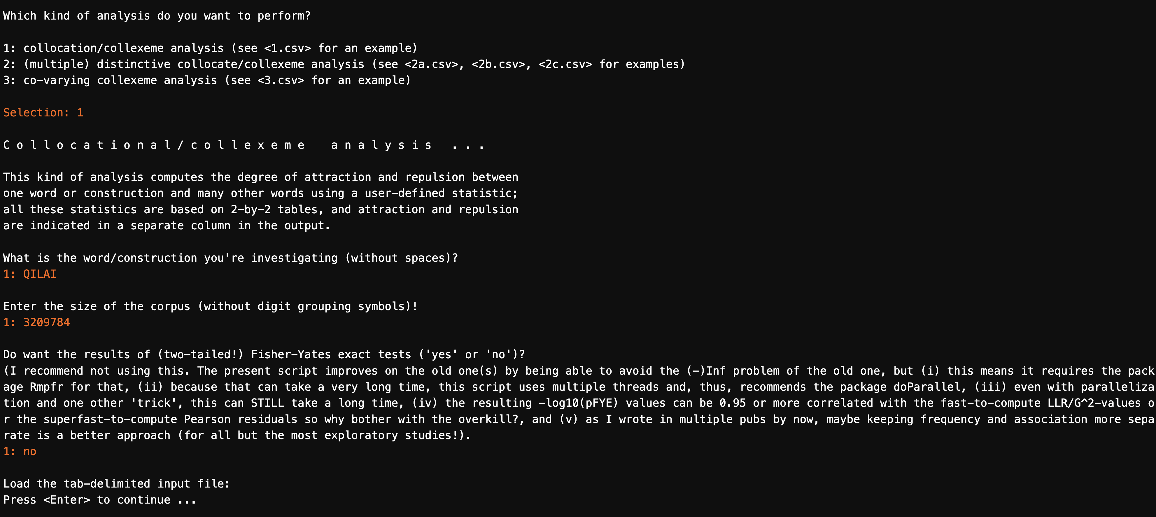
coll.analysis()coll.analysis() is an R program with interactive instructions.
When you run the analysis, you will be prompted with guided questions, to which you would need to fill in necessary information/answers in the R terminal.
For our current example, the answers to be entered for each prompt include:
analysis to perform: 1name of construction: QILAIcorpus size: 3209784Fisher-Yates: noTab-delimited input data:perfect.tsv
If everything works properly, you should get the output of the collexeme analysis as a CSV file in your working directory (a sample is provided in demo_data/qilai_results.csv).
8.4.4 Interpretations
Now we can load the CSV table and explore the results.
## load CSV
results <- read_tsv("demo_data/qilai_results.csv", locale = locale(encoding="UTF-8"))

## check top 50 based on LLR
results %>%
  filter(RELATION =="attraction") %>%
  arrange(desc(LLR)) %>%
  head(50) %>%
  select(WORD, LLR, everything())
The most important information from the result is the collostructional strength, namely LLR, which is a statistical measure indicating the association strength between each collexeme and the construction.
Please do check Stefanowitsch & Gries (2003) very carefully on how to interpret these numbers. For KL distance-based metrics such as KLDC2W, KLDW2C, please refer to Gries (2024) for more information.
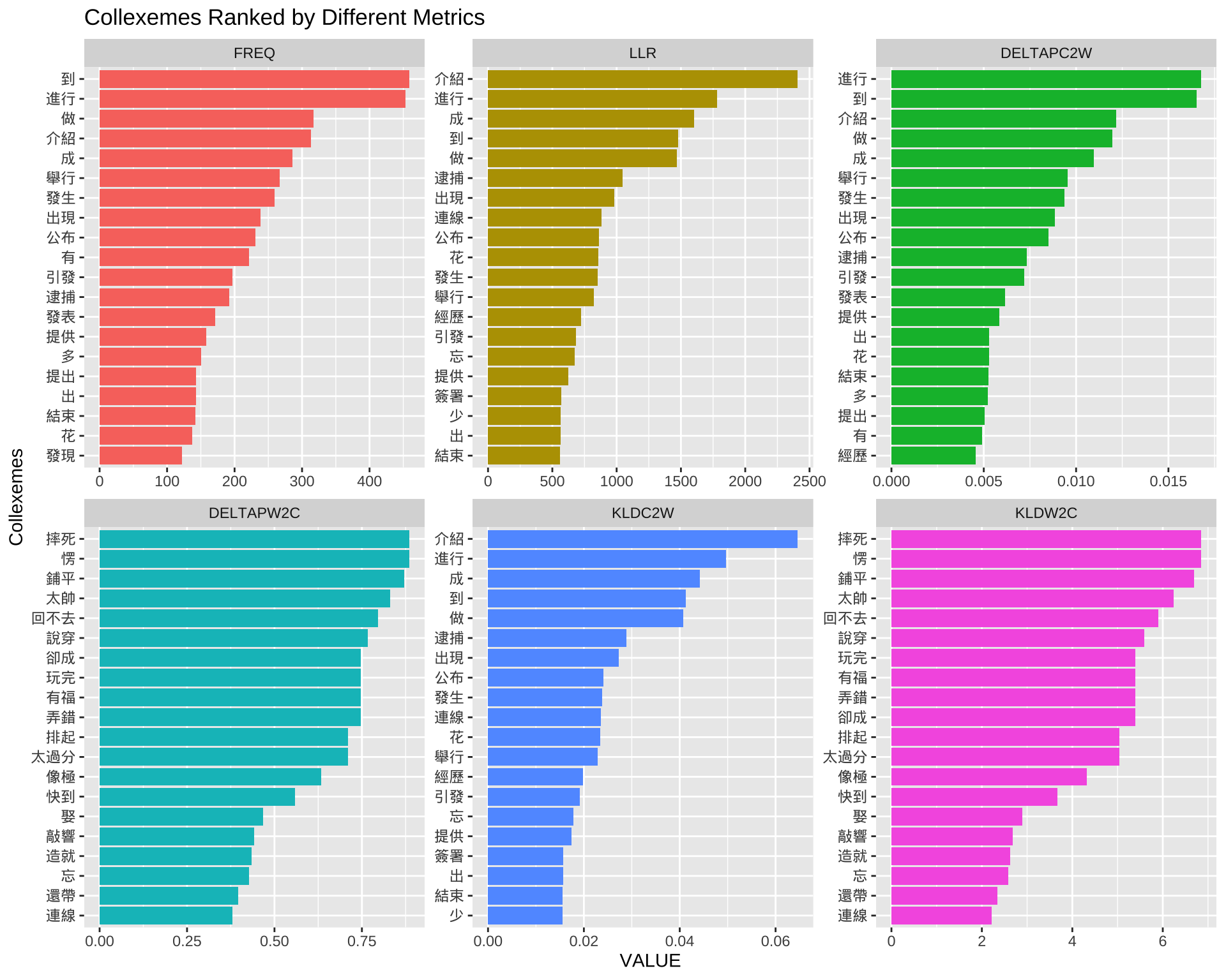
With the collexeme analysis statistics, we can therefore explore the top N collexemes according to specific association metrics.
Here we look at the top N collexemes according to different distributional/statistical metrics:
QILAI: co-occurrence frequency of word and constructionLLR: log-likelihood ratioDELTAPC2W: delta P (construction → word)DELTAPW2C: delta P (word → construction)KLDC2W: Kullback-Leibler Distance (construction → word)KLDW2C: Kullback-Leibler Distance (word → construction)
## from wide to long
results %>%
  filter(RELATION == "attraction") %>%
  filter(QILAI >= 5) %>%
  rename(FREQ = QILAI) %>%
  select(WORD,FREQ, LLR, DELTAPC2W, DELTAPW2C, KLDC2W, KLDW2C) %>%
  pivot_longer(
    cols = c("FREQ", "LLR", "DELTAPC2W", "DELTAPW2C", "KLDC2W", "KLDW2C"),
    names_to = "METRIC",
    values_to = "VALUE"
  ) %>%
  mutate(METRIC = factor(
    METRIC,
    levels = c("FREQ", "LLR", "DELTAPC2W", "DELTAPW2C", "KLDC2W", "KLDW2C")
  )) %>%
  group_by(METRIC) %>%
  top_n(20, VALUE) %>%
  ungroup %>%
  arrange(METRIC, desc(VALUE)) -> results_long

## plot
results_long %>%
    mutate(WORD = reorder_within(WORD, VALUE, METRIC)) %>%
    ggplot(aes(WORD, VALUE, fill=METRIC)) +
    geom_col(show.legend = F) +
    coord_flip() +
    facet_wrap(~METRIC,scales = "free") +
    tidytext::scale_x_reordered() +
    labs(x = "Collexemes",
         y = "VALUE",
         title = "Collexemes Ranked by Different Metrics")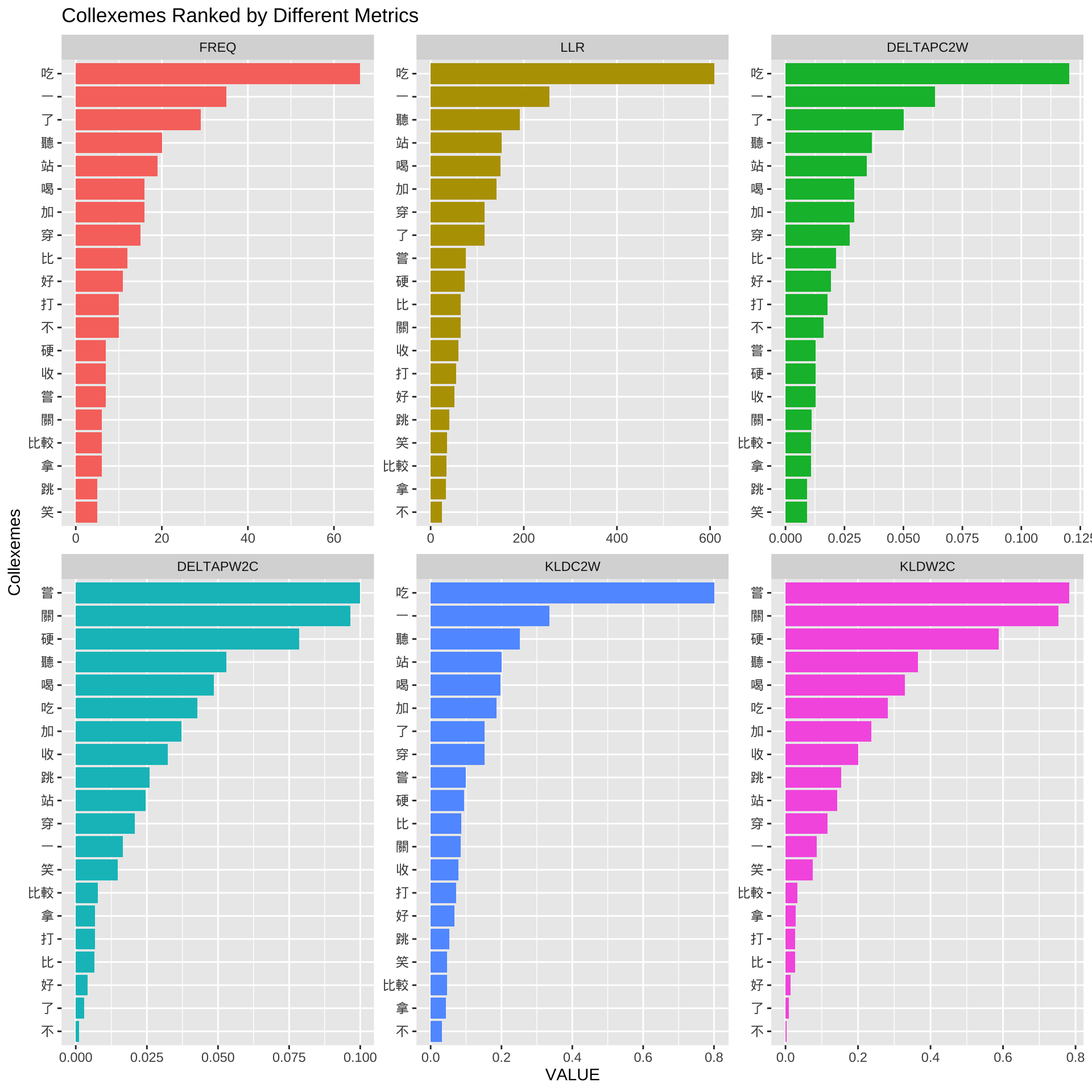
The bar plots above show the top N collexemes based on different metrics.
Please refer to the assigned readings on how to compute the collostrengths. Also, in Stefanowitsch & Gries (2003), please pay special attention to the parts where Stefanowitsch and Gries are arguing for the advantages of the collostrengths based on the Fisher Exact tests over the traditional raw frequency counts.
Specifically, delta P is a very unique association measure. It has received increasing attention in psycholinguistic studies. Please see Ellis (2006) and Gries (2013) for more comprehensive discussions on the issues of association’s directionality. I need everyone to have a full understanding of how delta p is computed and how we can interpret this association metric.
For KL Distance-based metrics, please check Gries (2024) for more comprehensive discussion.
Exercise 8.1 If we look at the top 10 collexemes ranked by the collostrength, we would see a few puzzling collexemes, such as 一, 了, 不. Please identify these puzzling construction tokens as concordance lines (using quanteda::kwic())and discuss their issues and potential solutions.
8.5 Distinctive Collexeme Analysis
8.5.1 Data
We can also use Stefan Gries’ script coll.analysis.r to perform a Distinctive Collexeme Analysis.
DCA is a useful method to study near synonymous constructions.
To illustrate this method, let’s use data from the following study:
Huang, P. W., & Chen, A. C. H. (2022). Degree adverbs in spoken Mandarin: A behavioral profile corpus-based approach to language alternatives. Concentric: Studies in Linguistics, 48(2), 285–322.
In this work, the focus is on differences among four Mandarin degree adverb constructions: 很 + X, 蠻/滿 + X, 超 + X, and 太 + X.
8.5.2 Analysis
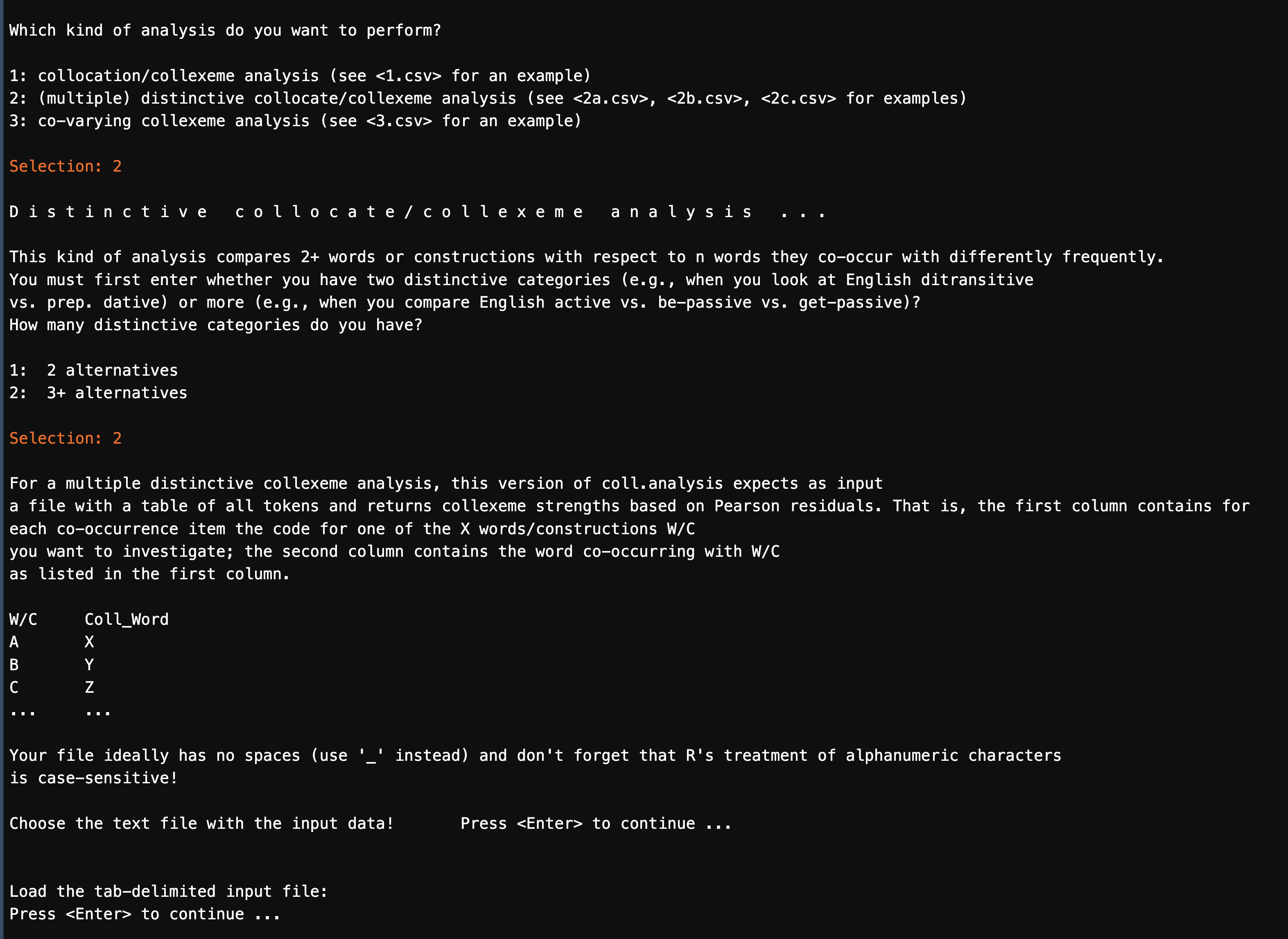
As before, we run the interactive function coll.analysis(). To use the program to conduct distinctive collexeme analysis, we need to provide necessary information/files as shown below.
analysis to perform: 2 (Distinctive Collexeme Analysis)
number of distinctive categories: 2 (or more if there are 3+ alternatives)
tab-delimited input data:<demo_data/input-distcollexeme.tsv>
For a Distinctive Collexeme Analysis, the input should be a data frame that lists each construction token in the corpus, with two key columns:
- The collexeme (the co-occurring word)
- The constructional element (the construction category being compared)
In our case, the constructional instances are the degree adverb constructions (e.g., 很 + X), and the collexemes are their co-occurring modifyees.
The following figure shows how these were annotated in concordance lines:
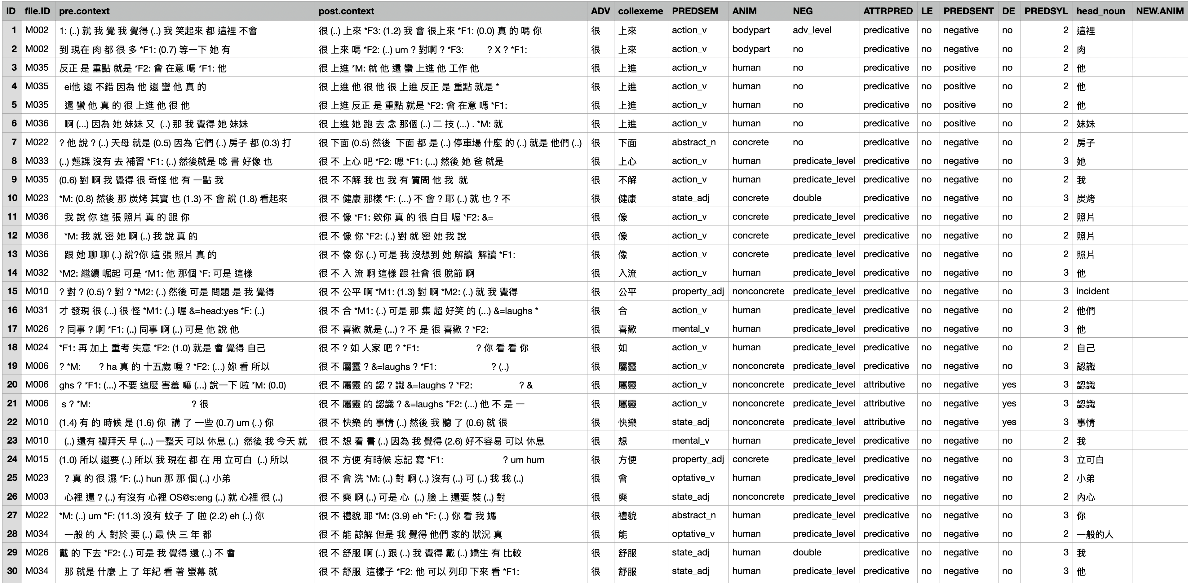
For Stefan’s script, we only need these two columns from the data: the collexemes and their associated constructional element.
With necessary information/files, we can run the DCA.
8.5.3 Interpretation
Once the script runs, it generates the results as a tab-delimited CSV file in the root directory.
An example output file is included in this project.
### Distinctive Collexeme Analysis: Results Exploration
dist_results <- read_tsv("demo_data/input-distcollexeme-results.csv", locale = locale(encoding = "UTF-8"))

dist_results
In distinctive collexeme analysis, the two columns mean:
SUMABSDEV shows how unevenly a word appears across the constructions. The larger this number, the more the word favors one construction over the others.
LARGESTPREF tells you which construction the word favors most — the one where it appears more often than expected.
So, if a collocate has a high SUMABSDEV and LARGESTPREF = A, it means the word occurs much more often in Construction A than chance would predict.
And our next step is to explore the semantic patterns from the output:
dist_results %>%
  group_by(LARGESTPREF) %>%
  top_n(10, SUMABSDEV) %>%
  select(COLLOCATE, SUMABSDEV, LARGESTPREF) %>%
  ungroup %>%
  arrange(LARGESTPREF) %>%
  mutate(COLLOCATE = reorder_within(COLLOCATE, within= LARGESTPREF, by=SUMABSDEV)) %>%
  ggplot(aes(COLLOCATE, SUMABSDEV, fill=SUMABSDEV)) +
    geom_col(show.legend = F) +
    scale_fill_distiller(palette="YlOrRd", direction=1)+
    coord_flip() +
    facet_wrap(~LARGESTPREF,scales = "free") +
    tidytext::scale_x_reordered() +
    labs(x = "COLLOCATE",
         y = "STRENGTH(SUMABSDEV)",
         title = "DISTINCTIVE COLLEXEMES")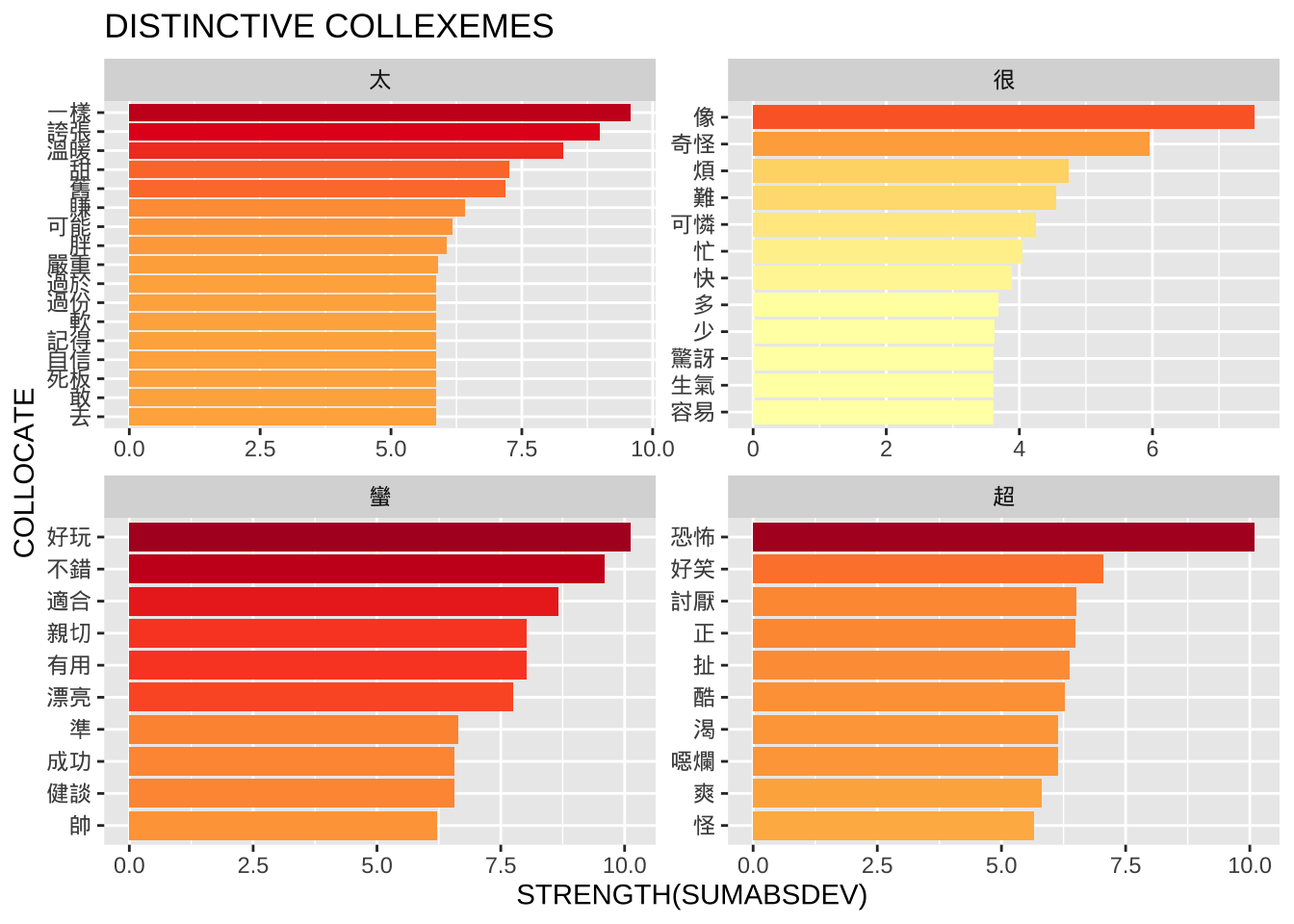
8.6 More Exercises
The following exercises should use the dataset Yet Another Chinese News Dataset from Kaggle.
The dataset is available on our dropbox demo_data/corpus-news-collection.csv.
The dataset is a collection of news articles in Traditional and Simplified Chinese, including some Internet news outlets that are NOT Chinese state media.
Exercise 8.2 Please conduct a collexeme analysis for the aspectual construction “X + 了” in Chinese.
Extract all tokens of this consturction from the news corpus and identify all words preceding the aspectual marker.
Based on the distributional information, conduct the collexemes analysis using the coll.analysis.r and present the collexemes that significantly co-occur with the construction “X + 了” in the X slot. Rank the collexemes according to the collostrength provided by Stefan Gries’ script.
When you tokenize the texts using jiebaR, you may run into an error message as shown below. If you do, please figure out what may have contributed to the issue and solve the problem on your own.

- It is suggested that you parse/tokenize the corpus data and create two additional columns to the text-based data frame —
text_id, andtext_tag. The following is an example of the first ten articles.
- A word frequency list of the top 100 words is attached below (word tokens that are pure whitespaces or empty strings were not considered)
After my data preprocessing and tokenization, here is relevant distributional information for
coll.analysis.r:- Corpus Size: 7898105
- Consturction Size: 25569
The output of the Collexeme Analysis (top 100 ranked by LLR) (
coll.analysis.r)
Exercise 8.3 Using the same Chinese news corpus—demo_data/corpus-news-collection.csv, please create a frequency list of all four-character words/idioms that are included in the four-character idiom dictionary demo_data/dict-ch-idiom.txt.
Please include both the frequency as well as the dispersion of each four-character idiom in the corpus. Dispersion is defined as the number of articles where it is observed.
Please arrange the four-character idioms according to their dispersion.
user system elapsed
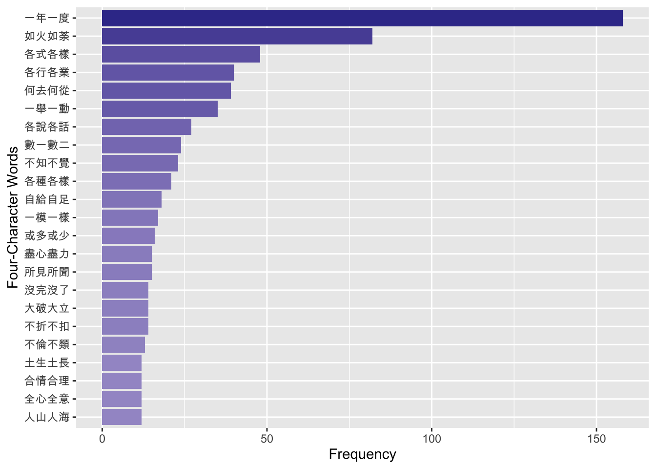
5.188 0.131 5.461 Exercise 8.4 Let’s assume that we are particularly interested in the idioms of the schema of X_X_, such as “一心一意”, “民脂民膏”, “滿坑滿谷” (i.e., idioms where the first character is the same as the third character).
Please find the top 20 frequent idioms of this schema and visualize their frequencies in a bar plot as shown below.
Exercise 8.5 Continuing the previous exercise, use the same set of idioms of the schema X_X_ and identify the X. Here we refer to the character X as the pivot of the idiom.
Please identify all the pivots for idioms of this schema which have at least two types of constructional variants in the corpus (i.e., its type frequency >= 2) and visualize their type frequencies as shown below.
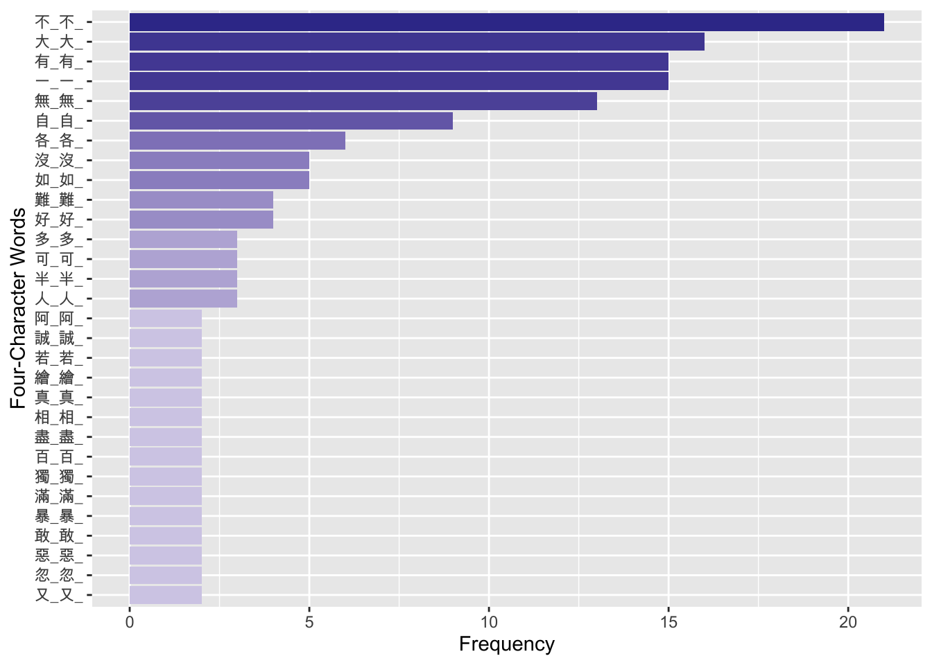
- For example, the type frequency of the most productive pivot schema, “不_不_”, is 21 in the news corpus. That is, there are 21 types of constructional variants of this schema with the pivot
不, as shown below:
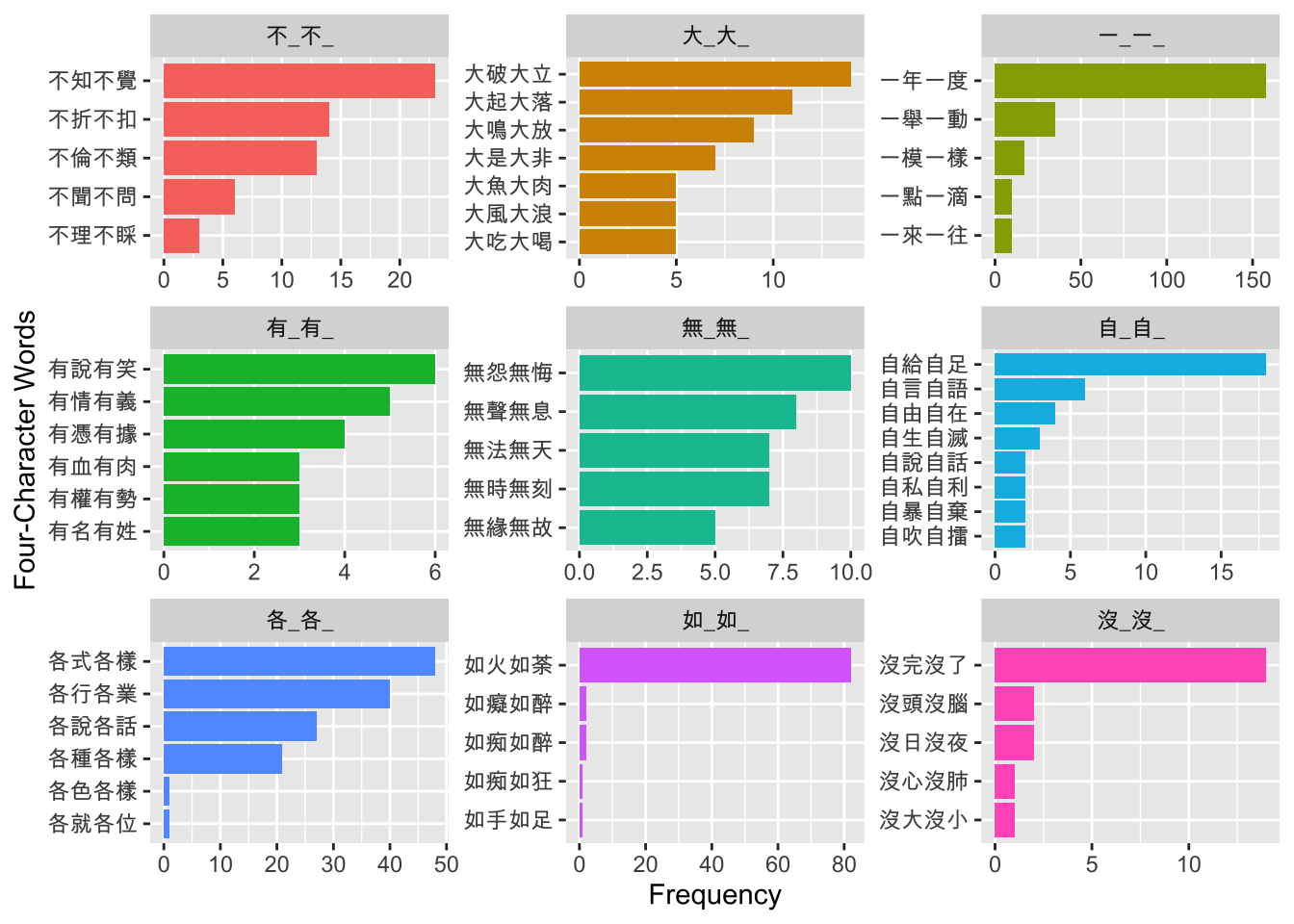
Exercise 8.6 Continuing the previous exercise, to further study the semantic uniqueness of each pivot schema, please identify the top 5 idioms of each pivot schema according to the frequencies of the idioms in the corpus.
Please present the results for schemas whose type frequencies >= 5 (i.e., the pivot schema has at least FIVE different idioms as its constructional instances).
Please visualize your results as shown below.
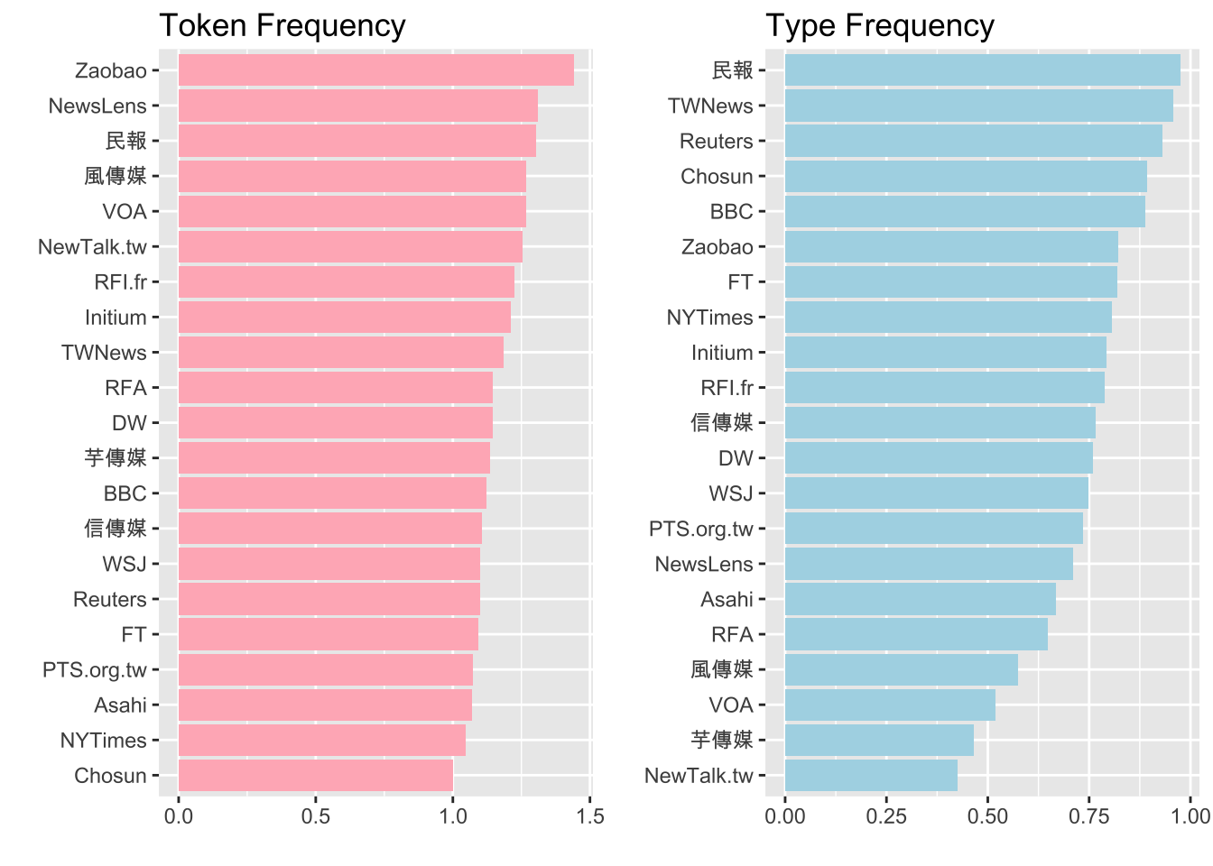
Exercise 8.7 Let’s assume that we are interested in how different media may use the four-character words differently.
Please show the average number of idioms per article by different media and visualize the results in bar plots as shown below.
The average number of idioms per article for each media source can be computed based on token frequency (i.e., on average how many idioms were observed in each article?) or type frequency (i.e., on average how many different idiom types were observed in each article?).
For example, there are 2529 tokens (1443 types) of idioms observed in the 1756 articles published by “Zaobao”.
- The average token frequency of idiom uses would be: 2529/1756 = 1.44;
- the average type frequency of idiom uses would be: 1443/1756 = 0.82.