Chapter 11 XML
This chapter shows you how to process the recently released BNC 2014, which is by far the largest representative collection of spoken English collected in UK. For the purpose of our in-class tutorials, I have included a small sample of the BNC2014 in our demo_data. However, the whole dataset is now available via the official website: British National Corpus 2014. Please sign up for the complete access to the corpus if you need this corpus for your own research.
11.1 BNC Spoken 2014
XML (the eXtensible Markup Language) is an effective format for text data storage, where the information of markup and annotation is added to the written texts in a structured way.
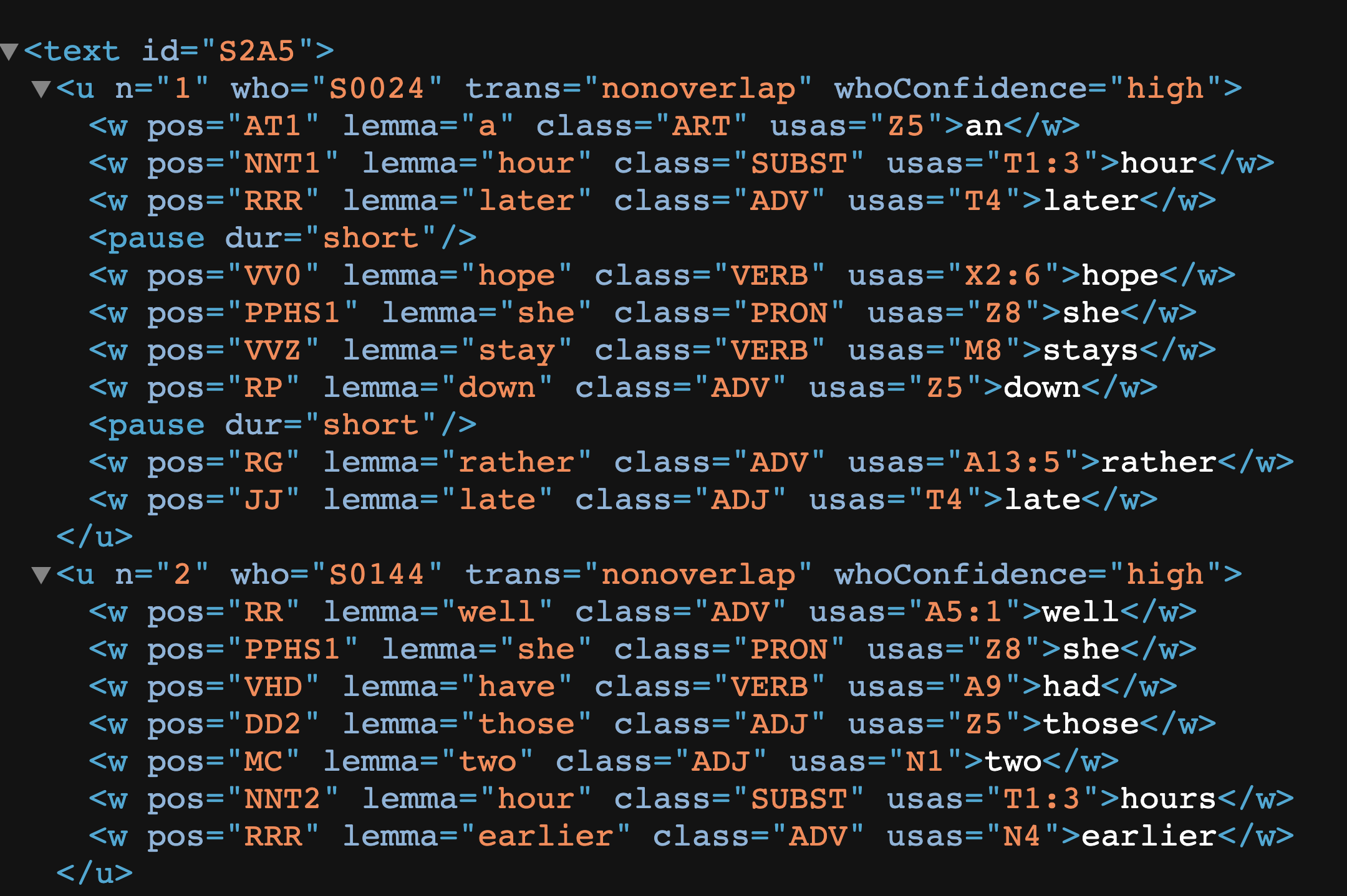
We can open an XML file with Google Chrome to take a look at its hierarchical structure.
Before we process the data, we need to understand the structure of the XML tags in the files. Usually we would start from the documentation of the corpus. Please read The BNC 2014: User Manual amd Reference Guide for more detail.
Other than that, the steps are pretty much similar to what we have learned before.
In this chapter, we will use xml2 to process XML files.
Please see Chapter 3.8.2 Some Notes on Handling XML Data in Gries (2017) for more discussions on XML processing. There are many R libraries supporting XML processing. The library rvest we use in Chapter 3 can also be used to process XML data. In addition to xml2 covered in this chapter, XML is another alternative for XML processing in R.
11.2 Processing one XML file
Each BNC XML file is like a tree structure. It starts with text node. Each text consists of utterance nodes u. Each utterance node consists of word nodes w or other para-linguistic feature nodes (e.g., pauses or vocal features).
Let’s see how we can process one single XML file from BNC2014 first. The steps include:
- Parse the XML file using
read_xml(); - Identity the XML root node using
xml_root(); - Extract all utterance nodes using
xml_find_all(); - Extract lexical units (word nodes) from each utterance node as well as their relevant annotations.
- Output everything as a data frame.
First, we read and parse an XML file using read_xml():
## read one XML
corp_bnc<-read_xml(x = "demo_data/corp-bnc-spoken2014-sample/S2A5-tgd.xml",
                   encoding = "UTF-8")
Second, we identity the XML root using xml_root():
[1] "text"Third, we extract all utterance nodes from the root using xml_find_all(), which supports the xpath query language for XML elements:
XPath is a query language that allows us to effectively identify specific elements from HTML/XML documents. We have used this in the task of web crawling in Chapter 3. Please read Chapter 4 XPath in Munzert et al. (2014) very carefully to make sure that you know how to use XPath.
## Extract <u> from XML
all_utterances <- xml_find_all(root, xpath = "//u")

## Check
print.AsIs(all_utterances[1])
[[1]]
{xml_node}
<u n="1" who="S0024" trans="nonoverlap" whoConfidence="high">
[1] <w pos="AT1" lemma="a" class="ART" usas="Z5">an</w>
[2] <w pos="NNT1" lemma="hour" class="SUBST" usas="T1:3">hour</w>
[3] <w pos="RRR" lemma="later" class="ADV" usas="T4">later</w>
[4] <pause dur="short"/>
[5] <w pos="VV0" lemma="hope" class="VERB" usas="X2:6">hope</w>
[6] <w pos="PPHS1" lemma="she" class="PRON" usas="Z8">she</w>
[7] <w pos="VVZ" lemma="stay" class="VERB" usas="M8">stays</w>
[8] <w pos="RP" lemma="down" class="ADV" usas="Z5">down</w>
[9] <pause dur="short"/>
[10] <w pos="RG" lemma="rather" class="ADV" usas="A13:5">rather</w>
[11] <w pos="JJ" lemma="late" class="ADJ" usas="T4">late</w>
attr(,"class")
[1] "xml_nodeset"[[1]]
{xml_node}
<u n="36" who="S0144" trans="nonoverlap" whoConfidence="high">
[1] <vocal desc="laugh"/>
[2] <pause dur="short"/>
[3] <w pos="DD1" lemma="that" class="ADJ" usas="Z8">that</w>
[4] <w pos="VBDZ" lemma="be" class="VERB" usas="A3">was</w>
[5] <w pos="AT1" lemma="a" class="ART" usas="Z5">a</w>
[6] <w pos="JJ" lemma="funny" class="ADJ" usas="E4:1">funny</w>
[7] <w pos="NN1" lemma="noise" class="SUBST" usas="X3:2">noise</w>
attr(,"class")
[1] "xml_nodeset"From the above output, we can see that under the <u> node, we may expect not only word nodes <w> but also non-word tokens, such as <pause .../>, <desc .../> (and many more).
Fourth, we need to extract all the children nodes (i.e., word and non-word nodes) from each utterance. This can be more complicated because each word node has a lot of annotations as attribute-value pairs in the start tag <w ATTRIBUTE = "VALUE"> XXX </w>.
Here let’s use the first utterance as an example. We can do the following:
- Extract all children nodes of the current utterance using
xml_children(); - Extract the tag name of each children node using
xml_name(); - Extract the corpus texts of each children node using
xml_text(); - Extract annotations (i.e., attributes) from each children node using
xml_attr();
[[1]]
{xml_node}
<u n="1" who="S0024" trans="nonoverlap" whoConfidence="high">
 [1] <w pos="AT1" lemma="a" class="ART" usas="Z5">an</w>
 [2] <w pos="NNT1" lemma="hour" class="SUBST" usas="T1:3">hour</w>
 [3] <w pos="RRR" lemma="later" class="ADV" usas="T4">later</w>
 [4] <pause dur="short"/>
 [5] <w pos="VV0" lemma="hope" class="VERB" usas="X2:6">hope</w>
 [6] <w pos="PPHS1" lemma="she" class="PRON" usas="Z8">she</w>
 [7] <w pos="VVZ" lemma="stay" class="VERB" usas="M8">stays</w>
 [8] <w pos="RP" lemma="down" class="ADV" usas="Z5">down</w>
 [9] <pause dur="short"/>
[10] <w pos="RG" lemma="rather" class="ADV" usas="A13:5">rather</w>
[11] <w pos="JJ" lemma="late" class="ADJ" usas="T4">late</w>

attr(,"class")
[1] "xml_nodeset"{xml_nodeset (11)}
[1] <w pos="AT1" lemma="a" class="ART" usas="Z5">an</w>
[2] <w pos="NNT1" lemma="hour" class="SUBST" usas="T1:3">hour</w>
[3] <w pos="RRR" lemma="later" class="ADV" usas="T4">later</w>
[4] <pause dur="short"/>
[5] <w pos="VV0" lemma="hope" class="VERB" usas="X2:6">hope</w>
[6] <w pos="PPHS1" lemma="she" class="PRON" usas="Z8">she</w>
[7] <w pos="VVZ" lemma="stay" class="VERB" usas="M8">stays</w>
[8] <w pos="RP" lemma="down" class="ADV" usas="Z5">down</w>
[9] <pause dur="short"/>
[10] <w pos="RG" lemma="rather" class="ADV" usas="A13:5">rather</w>
[11] <w pos="JJ" lemma="late" class="ADJ" usas="T4">late</w> [1] "w" "w" "w" "pause" "w" "w" "w" "w" "pause"
[10] "w" "w" [1] "an" "hour" "later" "" "hope" "she" "stays" "down"
[9] "" "rather" "late" ## Extract annotations of all children nodes
(token_pos <- xml_attr(all_children, attr="pos")) ## POS [1] "AT1" "NNT1" "RRR" NA "VV0" "PPHS1" "VVZ" "RP" NA
[10] "RG" "JJ" [1] "a" "hour" "later" NA "hope" "she" "stay" "down"
[9] NA "rather" "late" [1] "ART" "SUBST" "ADV" NA "VERB" "PRON" "VERB" "ADV" NA
[10] "ADV" "ADJ" [1] "Z5" "T1:3" "T4" NA "X2:6" "Z8" "M8" "Z5" NA
[10] "A13:5" "T4" ## Create DF
cur_utterance_df <- data.frame(
names = token_names,
texts = token_texts,
pos = token_pos,
lemma = token_lemma,
class = token_class,
usas = token_usas
)
cur_utterance_dfIn the result data frame above, we can see that there are quite a few rows which have NA values across all columns. Do you know why?
Take the first utterance node of the XML document for example. Each utterance node includes words as well as non-word tokens (i.e., para-linguistic annotations <pause .../>). We can retrieve:
- Strings of words in an utterance
- Lemma forms of all words in the utterance
- POS tags of all words in the utterance (BNC2014 uses UCREL CLAWS6 Tagset)
- Paralinguistic tags in the utterance
With the above example, it seems that we have completed the processing of the first utterance node and extracted most information we need from the first utterance. But there are still more we can extract from the utterance node:
- We can extract more information about the para-linguistic tags (e.g.,
<pause .../>,<vocal .../>), such as the pause duration, or other vocal descriptions.
[[1]]
{xml_node}
<u n="1" who="S0024" trans="nonoverlap" whoConfidence="high">
 [1] <w pos="AT1" lemma="a" class="ART" usas="Z5">an</w>
 [2] <w pos="NNT1" lemma="hour" class="SUBST" usas="T1:3">hour</w>
 [3] <w pos="RRR" lemma="later" class="ADV" usas="T4">later</w>
 [4] <pause dur="short"/>
 [5] <w pos="VV0" lemma="hope" class="VERB" usas="X2:6">hope</w>
 [6] <w pos="PPHS1" lemma="she" class="PRON" usas="Z8">she</w>
 [7] <w pos="VVZ" lemma="stay" class="VERB" usas="M8">stays</w>
 [8] <w pos="RP" lemma="down" class="ADV" usas="Z5">down</w>
 [9] <pause dur="short"/>
[10] <w pos="RG" lemma="rather" class="ADV" usas="A13:5">rather</w>
[11] <w pos="JJ" lemma="late" class="ADJ" usas="T4">late</w>

attr(,"class")
[1] "xml_nodeset"[[1]]
{xml_node}
<u n="36" who="S0144" trans="nonoverlap" whoConfidence="high">
[1] <vocal desc="laugh"/>
[2] <pause dur="short"/>
[3] <w pos="DD1" lemma="that" class="ADJ" usas="Z8">that</w>
[4] <w pos="VBDZ" lemma="be" class="VERB" usas="A3">was</w>
[5] <w pos="AT1" lemma="a" class="ART" usas="Z5">a</w>
[6] <w pos="JJ" lemma="funny" class="ADJ" usas="E4:1">funny</w>
[7] <w pos="NN1" lemma="noise" class="SUBST" usas="X3:2">noise</w>
attr(,"class")
[1] "xml_nodeset"- We can extract utterance-level metadata as well (i.e., the attributes of the
<u>node).- its unique index (
n) - speaker id (
who) - transition type (
trans, i.e., whether or not the transition between turns was overlapping) - attribution confidence (
whoconfidence, whether or not the transcriber was confident that they had correctly identified the speaker of the turn)
- its unique index (
[[1]]
            n           who         trans whoConfidence
          "1"       "S0024"  "nonoverlap"        "high"
Exercise 11.1 Now we know how to extract token-level information and utterance-level annotation from each utterance.
Please come up with a way to extract all relevant linguistic data from all utterances in the file demo_data/corp-bnc-spoken2014-sample/S2A5-tgd.xml, including their word and non-word tokens as well as their annotations and utterance-level metadata.
Ideally, the resulting data frame should consist of rows being the tokens of the utterances, and columns including the attributes and metadata of each token.
Specifically, for the word tokens, the data frame should include not only the word strings, but also the word-level annotations of part-of-speech tags, lemmas, and semantic tags (i.e., usas).
For non-word tokens (paralinguistic tags), the data frame should also include their information of attributes in a column, called notes.
Also, each token is connected to the utterance-level metadata, such as the utterance ID, speaker ID etc.
A sample data frame of the XML file is provided below (Only No 1 and 36 utterance nodes are included in the data frame for your reference).
11.3 Process the Whole Directory of BNC2014 Sample
11.3.1 Define Function
In Section 11.1, if you have figured out how to extract the token-based data frame from all utterances in an XML file, you can easily wrap the whole procedure as one function. With this function, we can repeat the same procedure for every XML file in BNC2014.
For example, let’s assume that we have defined a function:
This function takes one xml file as an argument and returns a token-based data frame, consisting of token strings and other relevant utterance-level and token-level information from the XML.
word_df <- read_xml_bnc2014(
  xmlfile = "demo_data/corp-bnc-spoken2014-sample/S2A5-tgd.xml")
word_df %>%
  filter(n %in% c("1","36"))
Exercise 11.2 Now your job is to create this function, read_xml_bnc2014(xmlfile = " ").
This function should take the path to one XML file as the input and return a token-based data frame of the XML file as the output.
11.3.2 Apply Function
Now we can utilize the self-defined function,
read_xml_bnc2014(), and process all XML files in thedemo_data/corp-bnc-spoken2014-sample/.Then we combine the individual
data.framereturned from each XML into a bigger one, i.e.,corp_bnc_token_df:
Please note that the following code chunk assumes that you have created the function read_xml_bnc2014() from the previous exercise.
## Get all XML filenames
bnc_flist <- dir("demo_data/corp-bnc-spoken2014-sample/",full.names = T)

## Extract token-based df from each XML
system.time(corp_bnc_list <- map(bnc_flist, read_xml_bnc2014))

## Combine all df's
corp_bnc_token_df <- bind_rows(corp_bnc_list)

## save file
write_csv(corp_bnc_token_df,
          file= "demo_data/data-corp-token-bnc2014.csv")
It takes a while to process/parse all the files included in the sample directory because we parse the entire XML file and extract almost everything (annotations + metadata) from the file.
You may store this corp_bnc_token_df data frame output for later use so that you don’t have to process the XML files every time you work with BNC2014.
The parsed token-based data frame of the BNC2014 is available in our demo_data/data-corp-token-bnc2014.csv. You can check if your output is the same as the CSV in the demo_data.
## Loading
corp_bnc_token_df <- read_csv(file = "demo_data/data-corp-token-bnc2014.csv",
                              locale = locale(encoding = "UTF-8"))

## Checking
corp_bnc_token_df %>%
  filter(xml_id == "S2A5-tgd.xml" & n %in% c("1","36"))
Also, in addition to <pause> and <vocal>, there are many other non-word tokens under the utterance nodes:
In the current design of read_xml_bnc2014(), we keep track of the annotations included in these non-word tokens in the notes column.
## Random sample of non-word tokens
corp_bnc_token_df %>%
  filter(!name %in% c("w")) %>%
  group_by(name) %>%
  sample_n(4)
You may check the BNC2014 documentation for more detail about the meanings of these XML tags.
11.4 Metadata
The best thing about BNC2014 is its rich demographic information related to the settings and speakers of the conversations. The whole corpus comes with two metadata sets:
bnc2014spoken-textdata.tsv: metadata for each text transcriptbnc2014spoken-speakerdata.tsv: metadata for each speaker ID
These two metadata sets allow us to get more information about each transcript as well as the speakers within those transcripts.
11.4.1 Text Metadata
There are two files that are relevant to the text metadata:
bnc2014spoken-textdata.tsv: This file includes the metadata information of each text filemetadata-fields-text.txt: This file includes the column names/meanings of the previous text metadata tsv, i.e.,bnc2014spoken-textdata.tsv.
## text metadata
bnc_text_meta <- read_tsv(
  file = "demo_data/corp-bnc-spoken2014-metadata/bnc2014spoken-textdata.tsv",
  col_names = FALSE,
  locale = locale(encoding = "UTF-8")
)
bnc_text_meta
## columns about text metadata
bnc_text_meta_names <- read_tsv(
file = "demo_data/corp-bnc-spoken2014-metadata/metadata-fields-text.txt",
skip = 1,
col_names = TRUE,
locale = locale(encoding = "UTF-8")
)
bnc_text_meta_names## Rename the columns of text metadata
names(bnc_text_meta) <- c("textid", bnc_text_meta_names$`XML tag`)
bnc_text_metaExercise 11.3 With the text metadata bnc_text_meta, please compute:
- the total amount of recording length for the current subset of BNC2014 (See the column
rec_length); - the average recording length of a transcript.
[1] "Total duration of the BNC2014 subset: 41 Days 03 Hours 50 Minutes 18 Seconds"[1] "On average, each transcript is about 47 Minutes 22.70 Seconds"11.4.2 Speaker Metadata
There are two files that are relevant to the speaker metadata:
bnc2014spoken-speakerdata.tsv: This file includes the demographic information of each speakermetadata-fields-speaker.txt: This file includes the column names/meanings of the previous speaker metadata tsv, i.e.,bnc2014spoken-speakerdata.tsv.
## speaker metadata
bnc_sp_meta <- read_tsv("demo_data/corp-bnc-spoken2014-metadata/bnc2014spoken-speakerdata.tsv",
                        col_names = FALSE,
                        locale = locale(encoding = "UTF-8"))
bnc_sp_meta
## columns about speaker metadata
bnc_sp_meta_names <- read_tsv("demo_data/corp-bnc-spoken2014-metadata/metadata-fields-speaker.txt",
skip = 1,
col_names = TRUE,
locale = locale(encoding = "UTF-8"))
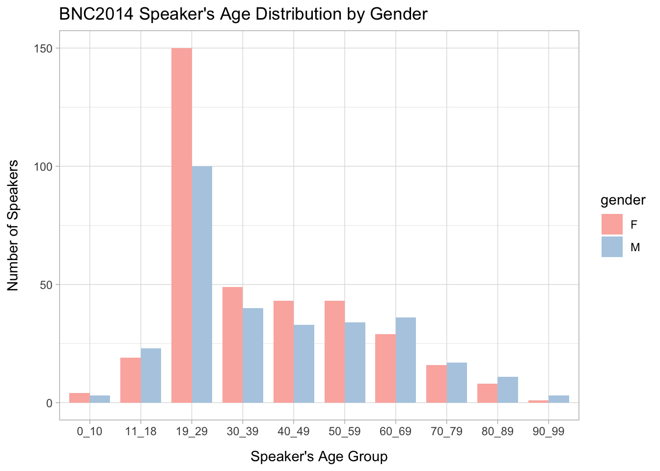
bnc_sp_meta_namesExercise 11.4 With the speaker metadata bnc_sp_meta, create a bar plot showing the age distribution (cf. agerange column) of the speakers by different genders in the current BNC2014 subset as shown below. (Disregard cases where the speaker’s age is unknown.)
11.5 BNC2014 for Socio-linguistic Variation
Now with both the text-level and speaker-level metadata, bnc_text_meta and bnc_sp_meta, we can easily connect the utterances to speaker and text profiles using their unique ID’s.
BNC2014 was born for the study of socio-linguistic variation. Here I would like to show you some naive examples, but you can get the ideas of what one can do with BNC2014.
11.6 Lexical Analysis
With the token-based data frame, we can perform lexical analysis on the lexical variations on specific social dimensions.
11.6.1 Word Frequency vs. Gender
In this section, I would like to demonstrate how to explore the gender differences in language.
Let’s assume that we like to know which adjectives are most frequently used by men and women.
## Extract adjectives and connect to speaker metadata
corp_bnc_adj_gender <- corp_bnc_token_df %>%  ## token-based DF
  filter(str_detect(pos, "^(JJ[RT]?$)")) %>%  ## adjectives
  left_join(bnc_sp_meta, by = c("who"="spid")) %>% ## link to metadata
  mutate(gender = factor(gender, levels=c("F","M"))) %>% ## factor gender
  filter(!is.na(gender)) ## remove gender-undefined tokens

## Check
corp_bnc_adj_gender %>% head(100)
11.6.2 Frequency and Keyword Analysis
After we extract word tokens that are adjectives, we can create a frequency list for each gender:
## create freq list by gender
freq_adj_by_gender <- corp_bnc_adj_gender %>%
  count(gender, lemma, sort = T)

## Show top 10 adjectives for each gender
freq_adj_by_gender %>%
  group_by(gender) %>%
  top_n(10, n) %>%
  ungroup %>%
arrange(gender, desc(n))- Female wordcloud
require(RColorBrewer)
require(wordcloud)
require(wordcloud2)

## Create female adjective word cloud
freq_adj_by_gender %>%
  filter(gender=="F") %>%
  top_n(100,n) %>%
  select(lemma, n) %>%
wordcloud2(size = 2, minRotation = -pi/2, maxRotation = -pi/2)- Male wordcloud
## Create male adjective word cloud
freq_adj_by_gender %>%
  filter(gender=="M") %>%
  top_n(100,n) %>%
  select(lemma, n) %>%
  wordcloud2(size = 2, minRotation = -pi/2, maxRotation = -pi/2)
Exercise 11.5 Which adjectives are more often used by male and female speakers? This should be a statistical problem. We can in fact extend our keyword analysis (cf. Chapter 6) to this question.
Please use the statistics of keyword analysis to find out the top 20 adjectives that are strongly attracted to female and male speakers according to G2 statistics. Please include in the analysis words whose frequencies >= 20 in the entire corpus.
Also, please note the problem of the NaN values out of the log().
- The top 50 adjectives by female speakers based on keyness
- The top 50 adjectives by male speakers based on keyness
11.7 Constructions Analysis
11.7.1 From Token-based to Turn-based Data Frame
We can also conduct analysis of specific constructions. We know that constructions often span word boundaries, but what we have right now is a token-based data frame of BNC2014.
For construction or multiword-unit analysis, we can convert the token-based DF into a turn-based DF, but keep necessary token-level annotations needed for your research project.
In this demonstration, I will show you how to convert the token-based DF into a turn-based DF, and keep the strings of word forms as well as parts-of-speech tags of words for each token.
- First, we transform the token-based data frame into a utterance-based token by nesting the token-level information of each utterance into a sub data frame.
This is our first time using nest() from tidyr, along with the group_by() function. The idea is simple: the grouping variables (i.e., utterance-level variables in our case) remain in the outer data frame and the others are nested (i.e., token-level variables in our case). I hope that the following animation provides a more comprehensive visual intuition of this nesting transformation.
## Load processed CSV of BNC2014
corp_bnc_token_df <- read_csv("demo_data/data-corp-token-bnc2014.csv",
                              locale = locale(encoding = "UTF-8"))

## Check
head(corp_bnc_token_df, 50)
## From token to utterance DF
corp_bnc_utterance_df <- corp_bnc_token_df %>%
select(-trans, -whoconfidence) %>% ## remove irrelevant columns
group_by(xml_id, n, who) %>% ## collapse utterance-level columns
nest %>% ## nest each utterance's token DF into sub-DF
ungroup
## check
corp_bnc_utterance_dfSecond, we create a function to process each utterance’s token-level data frame (the
datacolumn). In this self-defined function, we:- Extract the word forms (texts) and POS of each token
- Extract para-linguistic tag names. For non-word tokens, we use the name of the extra-linguistic XML tag, enclosed by
<and>, to represent the nature of the extra-linguistic annotations in the utterance. - Concatenate each utterance’s token-level information (texts + annotations + para-linguistic tags) into a long string
## Define a function
## to process the utterance's token-level data
extract_wordtag_string <- function(u_df){
  utterance_df <- u_df
  cur_text <-utterance_df$text  ## all word forms
  cur_pos <- utterance_df$pos ## all pos
  tag_index <-which(is.na(cur_text))  ## check paralinguistic index
  if(length(tag_index)>0){ ## retrieve paralinguistic
    cur_pos[tag_index]<- cur_text[tag_index] <- paste0("<",utterance_df$name[tag_index],">", sep ="")
  }
  ## concatenate and output
  paste(cur_text, cur_pos, sep = "_", collapse=" ")
} ## endfunc

## Example use
extract_wordtag_string(corp_bnc_utterance_df$data[[1]])
[1] "an_AT1 hour_NNT1 later_RRR <pause>_<pause> hope_VV0 she_PPHS1 stays_VVZ down_RP <pause>_<pause> rather_RG late_JJ"[1] "well_RR she_PPHS1 had_VHD those_DD2 two_MC hours_NNT2 earlier_RRR"- Finally, in the utterance-based data frame, we can apply the self-defined function
extract_wordtag_string()to each utterance’s token DF to obtain an enriched version of the utterance’s full texts.
## Applying function
corp_bnc_utterance_df %>%
  mutate(utterance = map_chr(data, extract_wordtag_string)) %>%
  select(-data) -> corp_bnc_utterance_df

## Check
corp_bnc_utterance_df %>% head(50)
If you would like to make use of more token-level information provided by BNC2014 (e.g. semantic annotations), you can revise the function extract_wordtag_string() and include these annotations before the string concatenation.
With the above utterance-based DF of the corpus, we can extract constructions or morphosyntactic patterns from the utterance column, utilizing the parts-of-speech tags provided by BNC2014.
11.7.2 Degree ADV + ADJ
In this section let’s look at the adjectives that are emphasized in conversations (e.g., too bad, very good, quite cheap) and examine how these emphatic adjectives may differ in speakers of different genders.
Here we define our patterns, utilizing the POS tags and the regular expressions: [^_]+_RG [^_]+_JJ.
- First, we extract the target patterns by converting the utterance-based DF into a pattern-based DF. We at the same time link each match with the speaker metadata.
## from utterance to pattern
## and linking speaker metadata
corp_bnc_pat_gender <- corp_bnc_utterance_df %>%
  unnest_tokens(pattern,  ## new unit
                utterance, ## old unit
                token = function(x)
                  str_extract_all(x, "[^_ ]+_RG [^_ ]+_JJ"),
                to_lower = FALSE) %>%
  left_join(bnc_sp_meta, by = c("who" = "spid"))


## Check
corp_bnc_pat_gender %>% head(100)- Second, we can create pattern frequencies by genders.
## Create frequency list
freq_pat_by_gender <- corp_bnc_pat_gender %>%
  mutate(pattern = str_replace_all(pattern, "_[^_ ]+","")) %>% # remove pos tags
  select(gender, pattern) %>%
  count(gender, pattern, sort=T)

## print top 100 by gender
freq_pat_by_gender %>%
  group_by(gender) %>%
  top_n(10,n) %>%
  ungroup %>%
arrange(gender, desc(n))- We can also create wordclouds for the patterns by gender
## word clouds
freq_pat_by_gender %>%
  filter(gender=="F") %>%
  top_n(100, n) %>%
  select(pattern, n) %>%
  wordcloud2(size = 0.9)
freq_pat_by_gender %>%
filter(gender=="M") %>%
top_n(100, n) %>%
select(pattern, n) %>%
wordcloud2(size = 0.9)Exercise 11.6 In the previous task, we have got the frequency list of the patterns (i.e., “Adverb + Adjective”) by gender, i.e., freq_pat_by_gender.
Please create a wide version of the frequency list, where each row is a pattern type and the columns include the frequencies of the patterns in male and female speakers, as well as the dispersion of the pattern in male and female speakers.
A sample has been provided below. Dispersion is defined as the number of (different) speakers who use the pattern at least once.
Exercise 11.7 So far we have been looking at the constructional schema of ADV + ADJ. Now let’s examine further how adjectives that are emphasized differ among speakers of different genders.
That is, do male speakers tend to emphasize adjectives that are different from those that are emphasized by females?
Now it should be clear to you that which adjectives are more likely to be emphasized by ADV in male and female utterances should be a statistical question.
Please use the statistics G2 from keyword analysis to find out the top 10 Adjectives that are strongly attracted to female and male speakers according to G2 statistics. Please include in the analysis adjectives whose dispersion >= 2 in the respective corpus, i.e., adjectives that have been used by at least TWO different male or female speakers.
Also, please note the problem of the NaN values out of the log().
- You first need to get the frequency list of the adjectives that occur in this constructional schema, ADV + ADJ:
- Then you convert the frequency list from a long format into a wide format for keyness computation.
- With the above distributional information, you can compute the keyness of the adjectives.
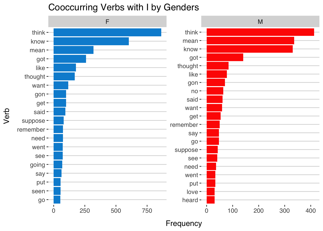
Exercise 11.8 Please analyze the verbs that co-occur with the first-person pronoun I in BNC2014 in terms of speakers of different genders. Please create a frequency list of the verbs that follow the first person pronoun I in demo_data/corp-bnc-spoken2014-sample. Verbs are defined as any words whose POS tag starts with VV. There can be up to two word tokens in-between the pronoun I and the verb (VV) (e.g., “I-canelled” pair in I_PPIS1 've_VH0 cancelled_VVN, “I-think” pair in I_PPIS1 do_VD0 n't_XX think_VVI).
Visualize the top 20 co-occurring verbs in a bar plot as shown below.
- All verb types on the top 100 lists of male and female speakers:
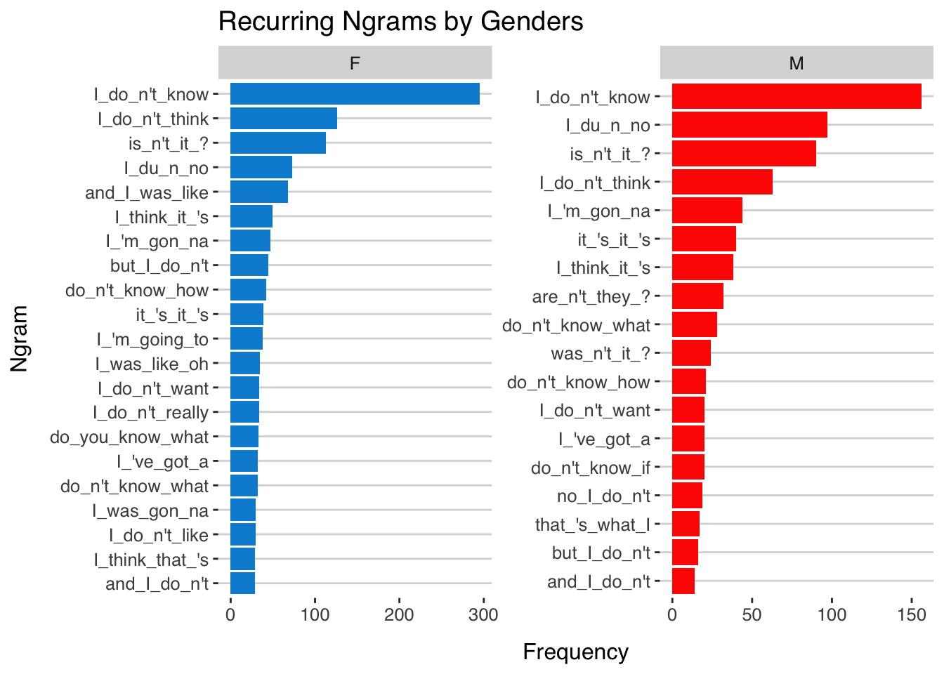
Exercise 11.9 Please analyze the recurrent four-grams used by male and female speakers by showing the top 20 four-grams used by males and females respectively ranked according to their frequencies.
Please disregard :
- Four-grams whose dispersion is \(\leq\) 10. Dispersion of four-grams is defined as the number of speakers who have used the four-gram in the corpus.
- Four-grams that include the non-word tokens (e.g., pauses or extralinguistic tags).
For those interested in analyzing spoken language data, R can directly read and process Praat TextGrid files. This is particularly useful if you want to integrate acoustic segmentation data into your corpus workflow without manual extraction. The rPraat library provides clean functionality to import TextGrids into R as structured data frames, allowing you to manipulate interval tiers (such as phone or word boundaries) and point tiers (such as pitch targets). Furthermore, the package allows you to extract acoustic parameters—including fundamental frequency (\(F_0\)) trajectories, formant values, and intensity contours—directly alongside your transcriptions, making it a powerful tool for large-scale phonetic and spoken corpus research.