Applications

Environment

## clear up memory
rm(list = ls(all=TRUE))

## loading necessary libraries
library(tidyverse)
library(quanteda)
library(quanteda.textplots)
library(quanteda.textstats)
library(readtext)
library(tidytext)
library(jiebaR)
library(wordcloud2)

## Windows-only
## Uncomment to set locale
# Sys.setlocale(category = "LC_ALL", locale = "cht")

## OS-specific fixing

## For Windows User
#Sys.setlocale(category = "LC_ALL", locale = "cht")

## Fix Chinese fonts in visualization
## Please replace your system-supported Chinese font
library(showtext)
#font_add("Arial Unicode MS", "Arial Unicode.ttf") ## <- replace your font
showtext_auto(enable = TRUE)

In this section, we will look at a few more examples of Chinese text processing based on the data set demo_data/song-jay-amei-v1.csv. It is a text collection of songs by Jay Chou and Amei.

Loading Data

We use the CSV version for illustration:

## loading CSV
corp_df_text <- read_csv(file = "demo_data/song-jay-amei-v1.csv", 
                         locale = locale(encoding = "UTF-8"))

## creating doc_id
corp_df_text <- corp_df_text %>%
  mutate(doc_id = row_number())

corp_df_text

Overview of the Corpus

The data set demo_data/song-jay-amei-v1.csv is a collection of songs by two artists, Jay Chou and Amei Chang.

A quick frequency counts of the songs by artists in the data set:

## Data set over view
str(corp_df_text)

spec_tbl_df [473 × 7] (S3: spec_tbl_df/tbl_df/tbl/data.frame)
 $ artist  : chr [1:473] "張惠妹" "張惠妹" "張惠妹" "張惠妹" ...
 $ title   : chr [1:473] "雙影" "Are You Ready" "偷故事的人" "壞的好人" ...
 $ lyricist: chr [1:473] "作詞：易家揚" "作詞：張雨生" "作詞：艾怡良" "作詞：小寒" ...
 $ composer: chr [1:473] "作曲：丁薇‭" "作曲：張雨生" "作曲：艾怡良" "作曲：黃晟峰" ...
 $ lyric   : chr [1:473] "若非狠下心拿什麼想妳\n想成了風雨‭　對不起\n保護一顆心看多了烏雲\n兩忘曾經裡　不怨妳\n‬\n心中有心語‭　‬‬妳我是雙影‭\n‬"| __truncated__ "Tell me baby are you ready天色已經黑\nTell me baby are you crazy用力說聲嘿\nTell me baby do you want it搖醒這世"| __truncated__ "當你走的那天 我不再說故事了\n不再編織起承轉合 也不用為結局苦惱了\n當你走的那天 你不再說故事了\n不再安排我的對白"| __truncated__ "紅燈黃昏狂奔 不顧輿論\n絶不能 讓心愛的他受冷\n不問緣分名稱 怕會扯分\n被一層 皮膚隔開的靈魂\n我的青春 不否認\n有"| __truncated__ ...
 $ gender  : chr [1:473] "female" "female" "female" "female" ...
 $ doc_id  : int [1:473] 1 2 3 4 5 6 7 8 9 10 ...
 - attr(*, "spec")=
  .. cols(
  ..   artist = col_character(),
  ..   title = col_character(),
  ..   lyricist = col_character(),
  ..   composer = col_character(),
  ..   lyric = col_character(),
  ..   gender = col_character()
  .. )
 - attr(*, "problems")=<externalptr> 

## Bar plot
corp_df_text %>%
  ggplot(aes(artist, fill=artist)) +
  geom_bar()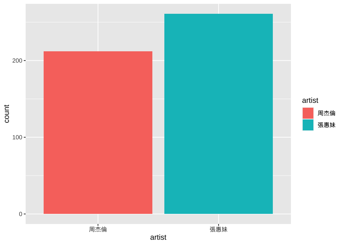 

Data Preprocessing (Cleaning)

Raw texts usually include a lot of noise. For example, texts may include control characters, redundant white-spaces, and duplicate line breaks. These redundant characters may have an impact on the word segmentation performance. It is often suggested to clean up the raw texts before tokenization.

## Define a function
normalize_document <- function(texts) {
  texts %>%
    str_replace_all("\\p{C}", " ") %>%  ## remove control chars
    str_replace_all("\\s+", "\n")  ## replace whitespaces with linebreak
}

## Example
corp_df_text$lyric[1]
[1] "若非狠下心拿什麼想妳\n想成了風雨‭　對不起\n保護一顆心看多了烏雲\n兩忘曾經裡　不怨妳\n‬\n心中有心語‭　‬‬妳我是雙影‭\n‬一半無情‭　另一半深情\n‬貪一點愛什麼痛也允許‭\n‬用懷疑交換‭　‬秘密\n寵愛和被忘‭　在心中交談‭(說來迷惘)\n妳作證我的冷暖‭　悲歡(夢短路長)\n妳拉我的手繡一件孤單(絲綢堆了月光)\n說用來取暖　誰敢\n命在誰命裡‭　‬愛恨是雙影\n一端美麗‭　另一端無語\n遠遠走來沒有字的未來\n被時間教會‭　也許\n情斷留情意‭　忘記是雙影\n一天冷淡另一天想起\n但願我們永遠走在光裡\n這一生如此‭　多雲\n這一生從此‭　無雲\n感謝\n好青年\n提供歌詞"

## Cleaned 
normalize_document(corp_df_text$lyric[1])
[1] "若非狠下心拿什麼想妳\n想成了風雨\n對不起\n保護一顆心看多了烏雲\n兩忘曾經裡\n不怨妳\n心中有心語\n妳我是雙影\n一半無情\n另一半深情\n貪一點愛什麼痛也允許\n用懷疑交換\n秘密\n寵愛和被忘\n在心中交談\n(說來迷惘)\n妳作證我的冷暖\n悲歡(夢短路長)\n妳拉我的手繡一件孤單(絲綢堆了月光)\n說用來取暖\n誰敢\n命在誰命裡\n愛恨是雙影\n一端美麗\n另一端無語\n遠遠走來沒有字的未來\n被時間教會\n也許\n情斷留情意\n忘記是雙影\n一天冷淡另一天想起\n但願我們永遠走在光裡\n這一生如此\n多雲\n這一生從此\n無雲\n感謝\n好青年\n提供歌詞"

## Apply cleaning to every document
corp_df_text$lyric <- normalize_document(corp_df_text$lyric)  

Initialize jiebaR

Because we use jiebaR for word tokenization, we first need to initialize the jiebaR models. Here we create two jiebaR models, one for word tokenization only and the other for parts-of-speech tagging.

## initialize jiebaR models

## for word segmentation only
my_seg <- worker(bylines = TRUE,
                 symbol = TRUE)

## for POS tagging
my_seg_pos <- worker(
  type = "tag",
  bylines = FALSE,
  symbol = TRUE
)

We can specify the path to the external user-defined dictionary in worker(..., user = "").

Alternatively, we can also add add-hoc new words to the jiebaR model. This can be very helpful when we spot any weird segmentation results in the output.

By default, new_user_word() assigns each new word with a default n tag.

#Add customized terms 
temp_new_words <-c("夢短路長")
new_user_word(my_seg, temp_new_words)

[1] TRUE

new_user_word(my_seg_pos, temp_new_words)

[1] TRUE

Tidytext Framework

The following examples demonstrate how to process the Chinese texts under the tidytext framework.

Recall the three important steps:

• Load the corpus data using readtext() and create a text-based data frame of the corpus;
• Initialize a jiebaR object using worker()
• Tokenize the text-based data frame into a word-based data frame using unnest_tokens();

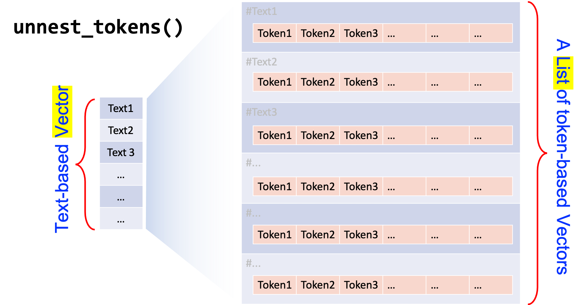
## Word Tokenization
corp_df_word <- corp_df_text %>%
  unnest_tokens(
    output = word, ## new unit name
    input = lyric, ## old unit name
    token = function (x)  ## tokenization method
      segment(x, jiebar = my_seg)
  ) %>%
  group_by(doc_id) %>%
  mutate(word_id = row_number()) %>%
  ungroup()

## Check
corp_df_word

Creating unique indices for your data is very important. In corpus linguistic analysis, we often need to keep track of the original context of the word, phrase or sentence in the concordances. All these unique indices (as well as the source text filenames) would make things a lot easier.

Also, if the metadata of the source documents are available, these unique indices would allow us to connect the tokenized linguistic units to the metadata information (e.g., genres, registers, author profiles) for more interesting analysis.

Therefore, after tokenization, we have obtained a word-based data frame of our corpus data.

Case Study: Word Frequency and Wordcloud

With a word-based data frame, we can easily create a word frequency list as well as a word cloud to have a quick overview of the word distribution of the corpus.

It should be noted that before creating the word frequency list, we often need to consider whether to remove unimportant word tokens. These unimportant tokens usually include:

• stopwords
• symbols and punctuation marks
• digits
• alphabets (e.g., English)

## load Chinese stopwords
stopwords_chi <- readLines("demo_data/stopwords-ch-jiebar-zht.txt", encoding = "UTF-8")

## create word freq list
corp_word_freq <- corp_df_word %>%
  filter(!word %in% stopwords_chi) %>% # remove stopwords
  filter(word %>% str_detect(pattern = "[\u4E00-\u9FFF]+")) %>% # including words consisting only of these Chinese chars
  count(word) %>%
  arrange(desc(n))

## Check top 50 words
head(corp_word_freq, 50)

## Create Word Cloud
library(wordcloud2)
corp_word_freq %>%
  filter(n > 20) %>% ## select words whose freq > 20
  filter(nchar(word) >= 2) %>% ## remove monosyllabic tokens
  wordcloud2(shape = "pentagon", size = 0.5)

We can represent any character in Unicode in the form of \uXXXX, where the XXXX refers to the coding numbers of the character in Unicode (UTF-8) in hexadecimal format.

In the above regular expression, the Unicode range [\u4E00-\u9FFF] refers to a set of frequently used Chinese characters. Therefore, the way we remove unimportant word tokens is to identify all word tokens consisting of these frequently used Chinese characters that fall within this Unicode range.

For more information related to the Unicode range for the punctuation marks in CJK languages, please see this SO discussion thread.

Case Study: Patterns

In this case study, we are looking at a more complex example. In corpus linguistic analysis, we often need to extract a particular pattern from the texts. In order to retrieve the target patterns at a high accuracy rate, we often need to make use of NLP tools to enrich the raw texts with more annotations. The most often-used information is the parts-of-speech tags of words.

In this example, we will demonstrate how to enrich our corpus data by adding POS tags to our current tidy corpus design.

Our steps are as follows:

1. Initialize jiebaR object, which performs not only word segmentation but also POS tagging;
2. Create a self-defined function to word-seg and pos-tag each text and combine all tokens, word/tag, into a long string for each text;
3. With the text-based data frame corp_df_text, create a new column, which includes the enriched version of each text, using mutate()

---

## Define a function to word-seg and pos-tag a text
tag_text <- function(x, jiebar) {
    segment(x, jiebar) %>% ## tokenize + POS-tagging
    paste(names(.), sep = "/", collapse = " ") ## reformat output
}

A quick example of the function’s usage:

## demo of the function `tag_text()`
tag_text(corp_df_text$lyric[1], 
         my_seg_pos)

[1] "若非/c 狠下/d 心/n 拿/v 什麼/r 想/v 妳/zg \n/x 想成/v 了/ul 風雨/n \n/x 對不起/l \n/x 保護/v 一顆/m 心看/x 多/m 了/ul 烏雲/nr \n/x 兩忘/x 曾經/d 裡/zg \n/x 不怨/v 妳/zg \n/x 心中/s 有/v 心語/n \n/x 妳/zg 我/r 是/v 雙影/n \n/x 一半/m 無情/n \n/x 另一半/d 深情/n \n/x 貪/v 一點/m 愛/zg 什麼/r 痛/a 也/d 允許/v \n/x 用/p 懷疑/v 交換/v \n/x 秘密/n \n/x 寵愛/v 和/c 被/p 忘/v \n/x 在/p 心中/s 交談/v \n/x (/x 說來/v 迷惘/a )/x \n/x 妳/zg 作證/v 我/r 的/uj 冷暖/an \n/x 悲歡/v (/x 夢短路長/n )/x \n/x 妳/zg 拉/v 我/r 的/uj 手繡/n 一件/m 孤單/a (/x 絲綢/n 堆/v 了/ul 月光/n )/x \n/x 說/zg 用來/v 取暖/v \n/x 誰/zg 敢/v \n/x 命/n 在/p 誰/zg 命裡/x \n/x 愛恨/a 是/v 雙影/n \n/x 一端/m 美麗/ns \n/x 另一端/i 無語/nz \n/x 遠遠/d 走來/v 沒有/v 字/n 的/uj 未來/t \n/x 被/p 時間/n 教會/n \n/x 也許/d \n/x 情斷/x 留情/v 意/n \n/x 忘記/v 是/v 雙影/n \n/x 一天/m 冷淡/a 另/r 一天/m 想起/v \n/x 但願/v 我們/r 永遠/d 走/v 在/p 光裡/x \n/x 這/zg 一生/m 如此/c \n/x 多雲/nr \n/x 這/zg 一生/m 從此/c \n/x 無/v 雲/ns \n/x 感謝/v \n/x 好/a 青年/t \n/x 提供/v 歌詞/n"

## Create a new column
## by applying `tag_text()` function to each text
corp_df_text <- corp_df_text %>%
  mutate(lyric_tag = map_chr(lyric, tag_text, my_seg_pos))

corp_df_text

---

Now we have obtained an enriched version of all the texts, we can make use of the POS tags for more linguistic analyses.

For example, we can examine the use of adjectives in lyrics.

The data retrieval procedure is now very straightforward: we only need to create a regular expression that matches our interested pattern and go through the enriched version of the texts (i.e., lyric_tag column in corp_df_text) to extract these matches with unnest_tokens().

1.Define a regular expression [^/\\s]+/a\\b for adjectives;

2.Use unnest_tokens() and str_extract_all() to extract target patterns and create a pattern-based data frame.

## define regex patterns
pat <- "[^/\\s]+/a\\b"

## extract patterns from corp
corp_df_pat <- corp_df_text %>%
  unnest_tokens(
    output = pat,  ## name for the new unit to be unnested
    input = lyric_tag, ## name for the old unit
    token = function(x)  ## unnesting method
      str_extract_all(x, pattern = pat)
  ) %>%
  select(doc_id, pat, artist, title)

corp_df_pat

---

Then we can further explore how different artists use the adjectives differently. We can identify the most frequently used top-20 adjectives for each artist and visualize the results in bar plots:

## Identify top 20 adjectives
corp_df_pat_top20 <- corp_df_pat %>%
  mutate(word = str_replace_all(pat, "/.+$","")) %>%  ## remove POS tags
  group_by(artist) %>% ## split DF by artist
  count(word, sort = T) %>% ## create pat freq list for each artist
  top_n(20, n) %>%  ## select top 20 for each artist
  ungroup %>% ## merge DF again
  arrange(artist, -n) ## sort result

## Check
corp_df_pat_top20

## Data Visualization: Bar plot 
corp_df_pat_top20 %>%
  mutate(word = reorder_within(word, n, artist)) %>%
  ggplot(aes(word, n, fill=artist)) +
  geom_bar(stat="identity")+ coord_flip()+
  facet_wrap(~artist,scales = "free_y") +
  scale_x_reordered() +
  labs(x = "Adjectives", y = "Frequency",
       title="Top 20 Adjectives of Each Artist's Songs")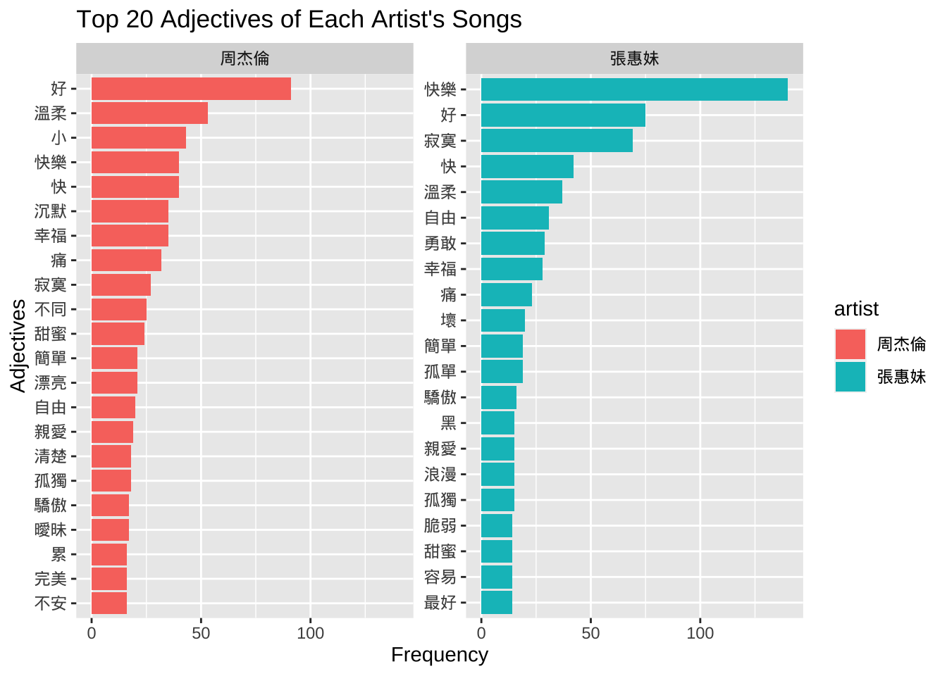

Case Study: Lexical Bundles

N-grams Extraction

With word boundaries, we can also analyze the recurrent multiword units in the corpus. In this example, let’s take a look at the recurrent four-word sequences (i.e., four-grams) in our corpus.

We define our own Chinese ngram tokenizer for unnest_tokens(). The Chinese ngram tokenization function should:

• Tokenize each raw text into word tokens;
• Create a set of ngrams from the word tokens of each text

## self defined ngram tokenizer
tokenizer_ngrams <-
  function(texts,
           jiebar,
           n = 2 ,
           skip = 0,
           delimiter = "_") {
    
    texts %>% ## given a vector of texts
      segment(jiebar) %>% ## word tokenization 
      as.tokens %>% ## list to tokens
      tokens_ngrams(n, skip, concatenator = delimiter)  %>%  ## ngram tokenization
      as.list ## tokens to list
  }

In the above self-defined ngram tokenizer, we make use of tokens_ngrams() in quanteda, which creates a set of ngrams from already tokenized text objects, i.e., tokens. Because this function requires a tokens object as the input, we need to do the class conversion via as.tokens() and as.list().

Take a look at the following examples for a quick overview of tokens_ngrams():

## Examples of quanteda's tokens_grams()
sents <- c("Jack and Jill went up the hill to fetch a pail of water",
           "Jack fell down and broke his crown and Jill came tumbling after")

sents_tokens <- tokens(sents) ## English tokenization
tokens_ngrams(sents_tokens, n = 2, skip = 0)

Tokens consisting of 2 documents.
text1 :
 [1] "Jack_and"  "and_Jill"  "Jill_went" "went_up"   "up_the"    "the_hill" 
 [7] "hill_to"   "to_fetch"  "fetch_a"   "a_pail"    "pail_of"   "of_water" 

text2 :
 [1] "Jack_fell"      "fell_down"      "down_and"       "and_broke"     
 [5] "broke_his"      "his_crown"      "crown_and"      "and_Jill"      
 [9] "Jill_came"      "came_tumbling"  "tumbling_after"

tokens_ngrams(sents_tokens, n = 2, skip = 1)

Tokens consisting of 2 documents.
text1 :
 [1] "Jack_Jill"  "and_went"   "Jill_up"    "went_the"   "up_hill"   
 [6] "the_to"     "hill_fetch" "to_a"       "fetch_pail" "a_of"      
[11] "pail_water"

text2 :
 [1] "Jack_down"     "fell_and"      "down_broke"    "and_his"      
 [5] "broke_crown"   "his_and"       "crown_Jill"    "and_came"     
 [9] "Jill_tumbling" "came_after"   

A quick example of how to use the self-defined function tokenizer_ngrams():

# examples
texts <- c("這是一個測試的句子",
           "這句子",
           "超短句",
           "最後一個超長的句子測試")

tokenizer_ngrams(
  texts = texts,
  jiebar = my_seg,
  n = 2,
  skip = 0, 
  delimiter = "_"
)

$text1
[1] "這是_一個" "一個_測試" "測試_的"   "的_句子"  

$text2
[1] "這_句子"

$text3
[1] "超短_句"

$text4
[1] "最後_一個" "一個_超長" "超長_的"   "的_句子"   "句子_測試"

tokenizer_ngrams(
  texts = texts,
  jiebar = my_seg,
  n = 2,
  skip = 1, 
  delimiter = "_"
)

$text1
[1] "這是_測試" "一個_的"   "測試_句子"

$text2
character(0)

$text3
character(0)

$text4
[1] "最後_超長" "一個_的"   "超長_句子" "的_測試"  

tokenizer_ngrams(
  texts = texts,
  jiebar = my_seg,
  n = 5,
  skip=0,
  delimiter = "_"
)

$text1
[1] "這是_一個_測試_的_句子"

$text2
character(0)

$text3
character(0)

$text4
[1] "最後_一個_超長_的_句子" "一個_超長_的_句子_測試"

---

With the above self-defined Chinese ngram tokenizer, we can now perform the ngram tokenization on our corpus. The principle is the same:

1. We transform the text-based data frame into an ngram-based data frame using unnest_tokens(...) with the self-defined tokenization function tokenizer_ngrams();

2. We remove empty and unwanted n-grams entries:

   • Empty ngrams due to short texts
   • Ngrams spanning punctuation marks, symbols, or paragraph breaks
   • Ngrams including alphanumeric characters

## Ngram tokenization
## from text-based to ngram-based DF
corp_df_ngram <- corp_df_text %>%
  unnest_tokens(
    ngram, ## name for the new unit to be unnested
    lyric,  ## name for the old unit
    token = function(x) ## unnesting method
      tokenizer_ngrams(
        texts = x,
        jiebar = my_seg,
        n = 4,
        skip = 0,
        delimiter = "_"
      )
  ) %>%
  select(doc_id, ngram, artist, title, lyricist)


## remove unwanted ngrams
corp_df_ngram_2 <- corp_df_ngram %>%
  filter(nzchar(ngram)) %>% ## empty strings
  filter(!str_detect(ngram, "[^\u4E00-\u9FFF_]")) ## include ngrams consisting of Chinese characters + _

## check
head(corp_df_ngram_2,50)

Frequency and Dispersion

Now we can compute two important distributional properties of these 4-grams (Biber, Conrad, and Cortes 2004):

• The token frequency of the 4-gram;
• The number of different texts where the 4-gram is observed (i.e., dispersion)

We set cut-offs for four-grams at: dispersion >= 3 (i.e., four-grams that occur in at least three different songs)

## Compute ngram's frequency and dispersion
corp_ngram_dist <- corp_df_ngram_2 %>%
  group_by(ngram) %>%
  summarize(freq = n(), 
            dispersion = n_distinct(doc_id)) %>%
  filter(dispersion >= 3) %>%
  ungroup

## Check DF arranged by dispersion
corp_ngram_dist %>%
  arrange(desc(dispersion)) %>% head(50)

We can also look at four-grams with particular lexical words:

## Check ngrams with a specific word
corp_ngram_dist %>%
  filter(str_detect(ngram, "我")) %>%
  arrange(desc(dispersion))

corp_ngram_dist %>%
  filter(str_detect(ngram, "你")) %>%
  arrange(desc(dispersion))

corp_ngram_dist %>%
  filter(str_detect(ngram, "媽媽")) %>%
  arrange(desc(dispersion))

Quanteda Framework

Now let’s look at a few examples of processing the data with the quanteda framework.

For Chinese data, the most important base unit in Quanteda is the tokens object. So first we need to create the tokens object based on the jiebaR tokenization method.

## create tokens based on self-defined segmentation
corp_tokens <- as.tokens(segment(corp_df_text$lyric, my_seg))

## add document-level metadata 
docvars(corp_tokens) <- corp_df_text[, c("artist","lyricist","composer","title","gender")]

## check 1st doc
corp_tokens[[1]]

  [1] "若非"     "狠下"     "心"       "拿"       "什麼"     "想"      
  [7] "妳"       "\n"       "想成"     "了"       "風雨"     "\n"      
 [13] "對不起"   "\n"       "保護"     "一顆"     "心看"     "多"      
 [19] "了"       "烏雲"     "\n"       "兩忘"     "曾經"     "裡"      
 [25] "\n"       "不怨"     "妳"       "\n"       "心中"     "有"      
 [31] "心語"     "\n"       "妳"       "我"       "是"       "雙影"    
 [37] "\n"       "一半"     "無情"     "\n"       "另一半"   "深情"    
 [43] "\n"       "貪"       "一點"     "愛"       "什麼"     "痛"      
 [49] "也"       "允許"     "\n"       "用"       "懷疑"     "交換"    
 [55] "\n"       "秘密"     "\n"       "寵愛"     "和"       "被"      
 [61] "忘"       "\n"       "在"       "心中"     "交談"     "\n"      
 [67] "("        "說來"     "迷惘"     ")"        "\n"       "妳"      
 [73] "作證"     "我"       "的"       "冷暖"     "\n"       "悲歡"    
 [79] "("        "夢短路長" ")"        "\n"       "妳"       "拉"      
 [85] "我"       "的"       "手繡"     "一件"     "孤單"     "("       
 [91] "絲綢"     "堆"       "了"       "月光"     ")"        "\n"      
 [97] "說"       "用來"     "取暖"     "\n"       "誰"       "敢"      
[103] "\n"       "命"       "在"       "誰"       "命裡"     "\n"      
[109] "愛恨"     "是"       "雙影"     "\n"       "一端"     "美麗"    
[115] "\n"       "另一端"   "無語"     "\n"       "遠遠"     "走來"    
[121] "沒有"     "字"       "的"       "未來"     "\n"       "被"      
[127] "時間"     "教會"     "\n"       "也許"     "\n"       "情斷"    
[133] "留情"     "意"       "\n"       "忘記"     "是"       "雙影"    
[139] "\n"       "一天"     "冷淡"     "另"       "一天"     "想起"    
[145] "\n"       "但願"     "我們"     "永遠"     "走"       "在"      
[151] "光裡"     "\n"       "這"       "一生"     "如此"     "\n"      
[157] "多雲"     "\n"       "這"       "一生"     "從此"     "\n"      
[163] "無"       "雲"       "\n"       "感謝"     "\n"       "好"      
[169] "青年"     "\n"       "提供"     "歌詞"    

Case Study: Concordances with kwic()

With this tokens object, we can perform the concordance analysis with kwic() and create a dispersion plot of the keyword.

## keyword-in-context
kwic(corp_tokens, "快樂", window = 10)

## Create dispersion plot based on kwic
textplot_xray(
  kwic(corp_tokens, "雙截棍"))

Because we have also added the document-level information, we can utilize these document-level variables and perform more interesting analysis.

For example, we can examine the concordance lines of a keyword in a subset of the corpus. In the following code chunk, we examine the concordance lines of 快樂 and 難過 in songs written by 方文山.

## Subsetting tokens
corp_tokens_subset <-tokens_subset(corp_tokens, ## tokens
                                   str_detect(lyricist, "方文山")) ## subsetting rule

## Creating dispersion plot based on kwic
textplot_xray(
  kwic(corp_tokens_subset, "快樂"),
  kwic(corp_tokens_subset, "難過"))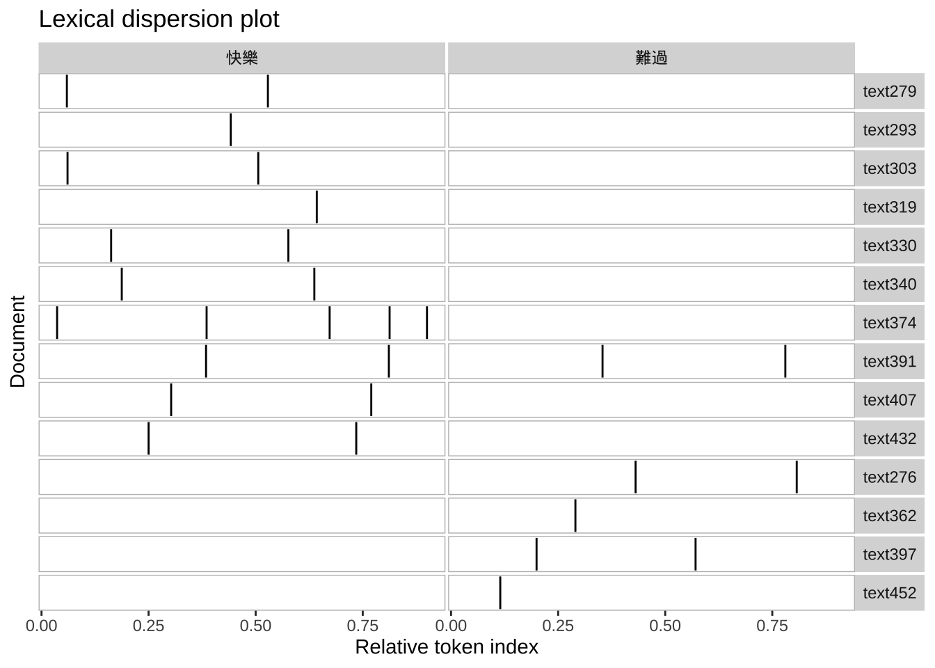

Case Study: Comparison Word Cloud

In quanteda, we can quickly create a comparison word cloud, showing the the differences of the lexical distributions in different corpus subsets. For example, we can create a comparison word cloud to show the lexical differences of Jay’s and Amei’s songs.

## Create comparison word clouds
corp_tokens %>% 
  dfm() %>% ## from tokens to dfm objects
  dfm_remove(pattern= stopwords_chi, ## remove stopwords
             valuetype="fixed") %>% 
  dfm_keep(pattern = "[\u4E00-\u9FFF]+",  ## include words consisting of freq Chinese chars
           valuetype= "regex") %>% 
  dfm_group (groups = artist) %>% ## group by artist
  dfm_trim(min_termfreq = 10, ## distributional cutoffs
           min_docfreq = 2,
           verbose = F) %>%
  textplot_wordcloud(comparison=TRUE,
                     min_size = 0.8,
                     max_size = 4,
                     color = c("navyblue","gold"))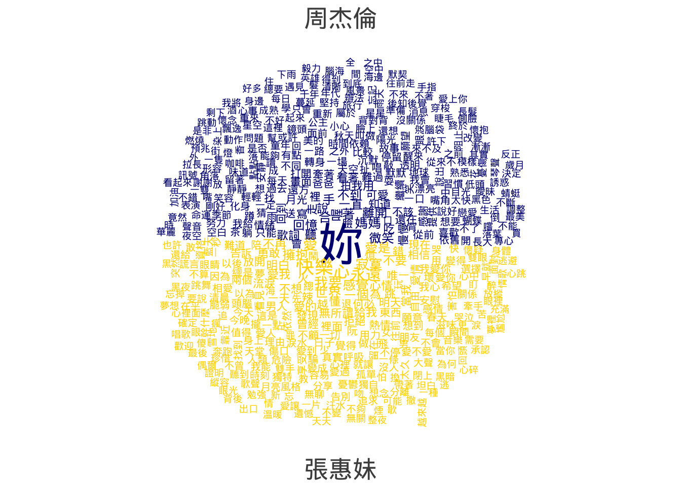

Case Study: Collocations

## extract collocations
corp_collocations <- corp_tokens %>%
  tokens_keep(pattern = "[\u4E00-\u9FFF]+",  ## include words consisting of freq Chinese chars
              valuetype= "regex") %>%
  textstat_collocations(
    size = 2, 
    min_count = 10)

## Check top 20 collocations in the corpus
top_n(corp_collocations, 20, z)

Conclusion

Tokenization is an important step in Chinese text processing. We may need to take into account many factors when determining the right tokenization method, including:

1. What is the base unit we would like to work with? Texts? Paragraphs? Chunks? Sentences? N-grams? Words?
2. Do we need an enriched version of the raw texts, e.g., the parts-of-speech tags of words in the later analysis?
3. Do we need to include non-word tokens such as symbols, punctuation marks, digits, or alphabets in the analysis?
4. Do we need to remove semantically irrelevant/unimportant words, i.e., stopwords?
5. Do we have many domain-specific words in our corpus (e.g., terminology, proper names)?

The answers to the above questions would give us more clues on how to determine the most effective tokenization methods for the data.

---

Thank you!

Questions?

References

Biber, Douglas, Susan Conrad, and Viviana Cortes. 2004. “If You Look at…: Lexical Bundles in University Teaching and Textbooks.” Applied Linguistics 25 (3): 371–405.